Impact of viscosity on creeping viscous fluid flow through a permeable slit: a study for the artificial kidneys

Khadija Maqbool; Hira Mehboob; Abdul Majeed Siddiqui; Khadija Maqbool; Hira Mehboob; Abdul Majeed Siddiqui

doi:10.3934/biophy.2022026

AIMS Biophysics

2022, Volume 9, Issue 4: 308-329. doi: 10.3934/biophy.2022026

Previous Article Next Article

Research article Special Issues

Impact of viscosity on creeping viscous fluid flow through a permeable slit: a study for the artificial kidneys

1.
Department of Mathematics & Statistics, International Islamic University, Islamabad 44000, Pakistan
2.
Department of Mathematics Pennsylvania State University, York Campus, York, PA 17403, USA

Received: 10 August 2022 Revised: 27 October 2022 Accepted: 31 October 2022 Published: 08 November 2022

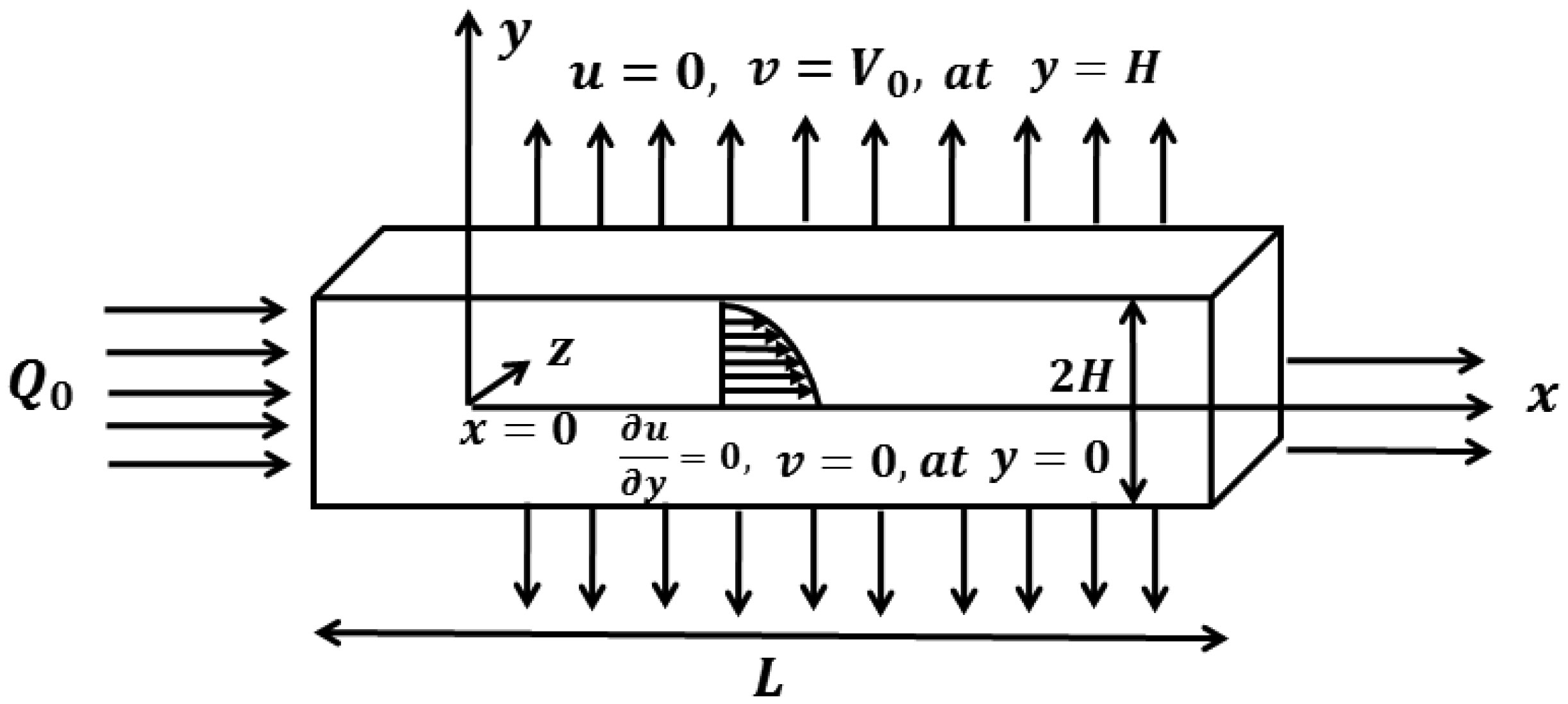
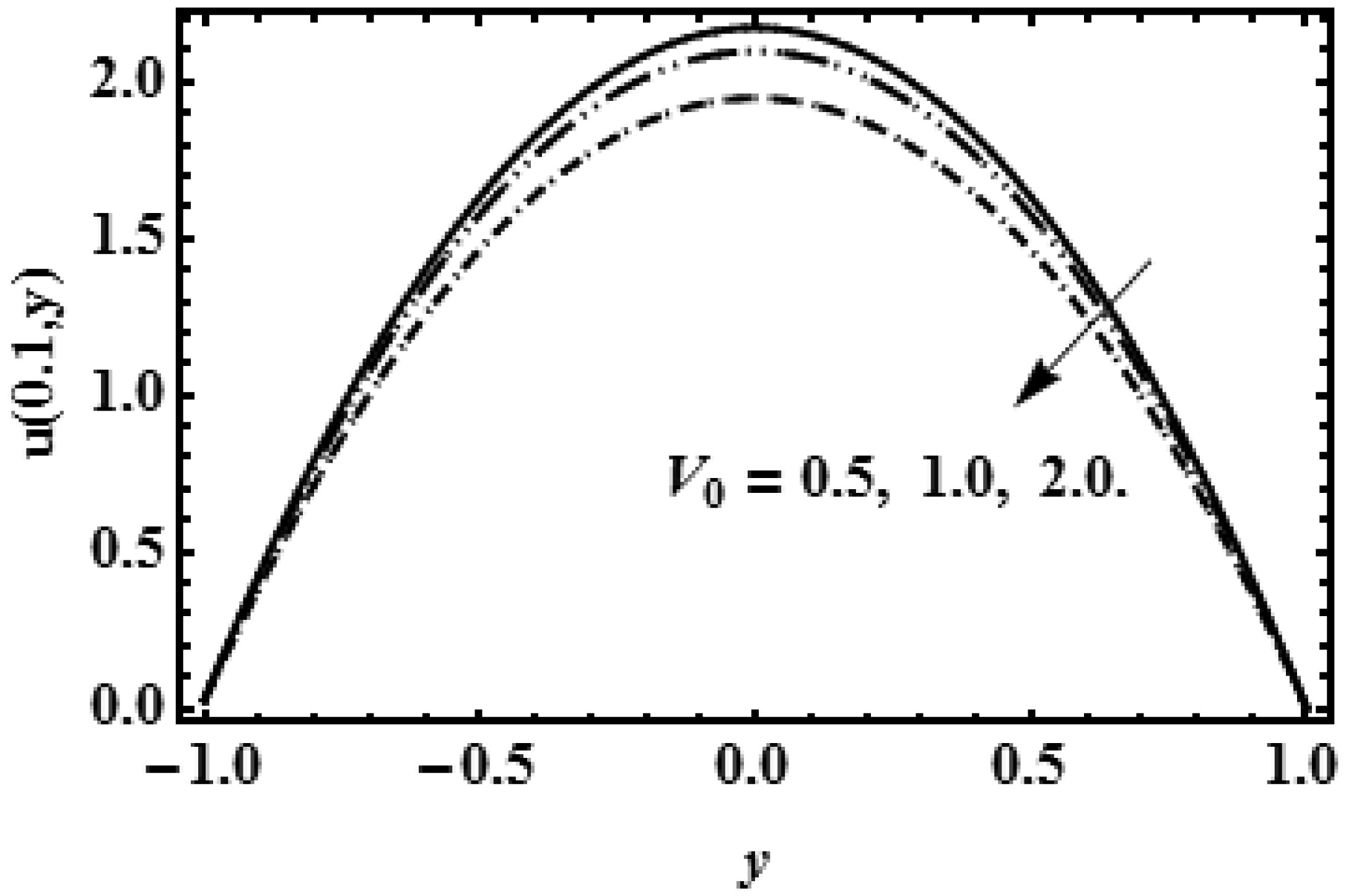
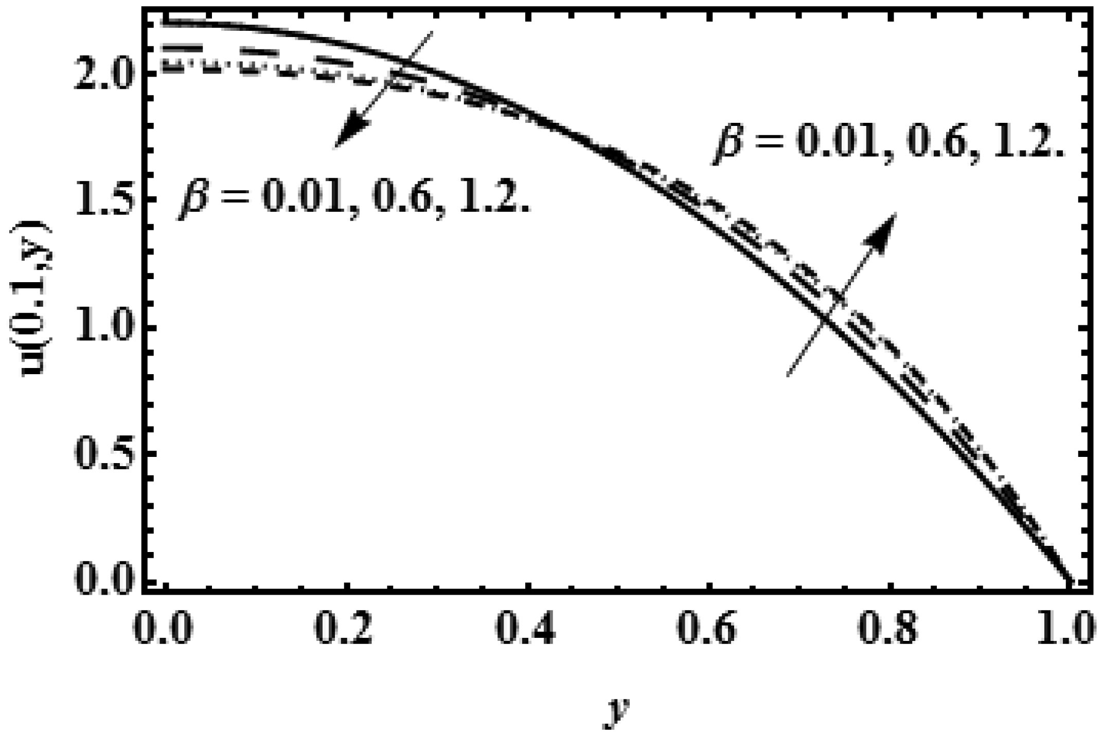
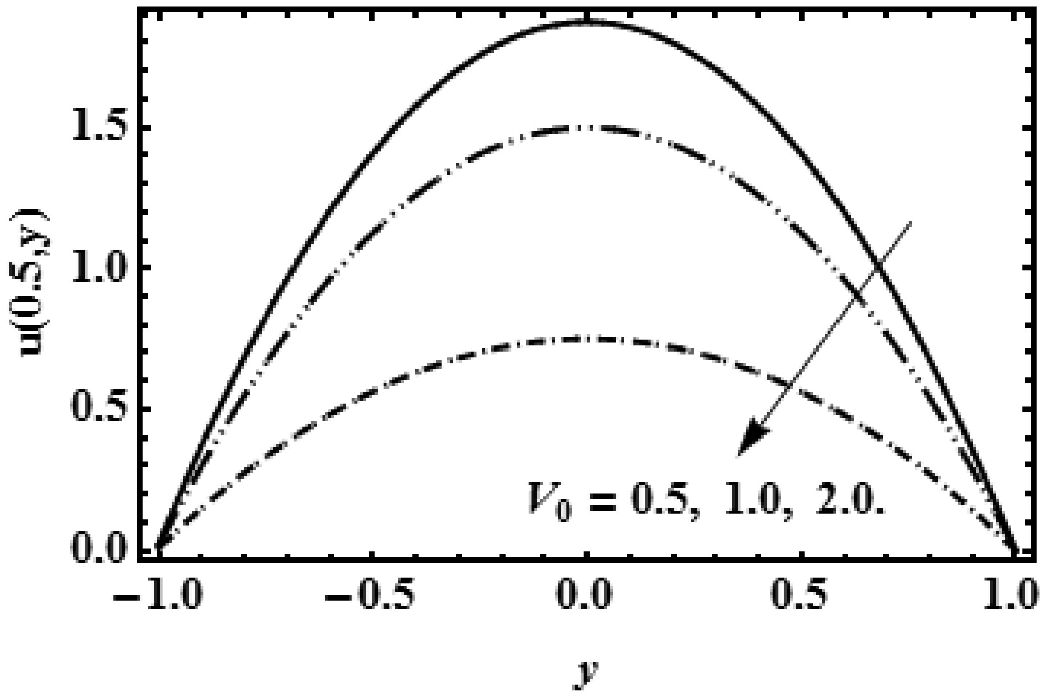
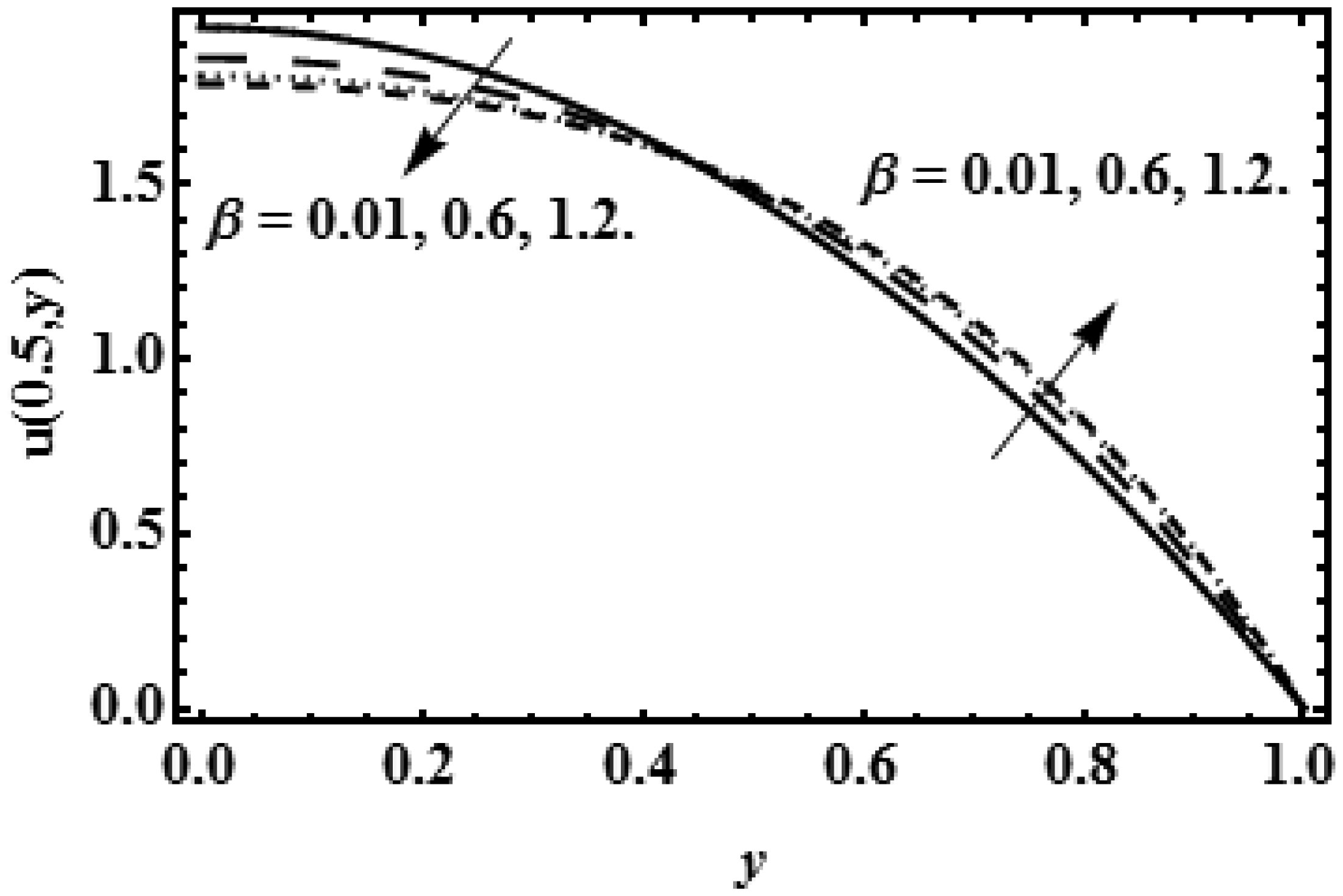
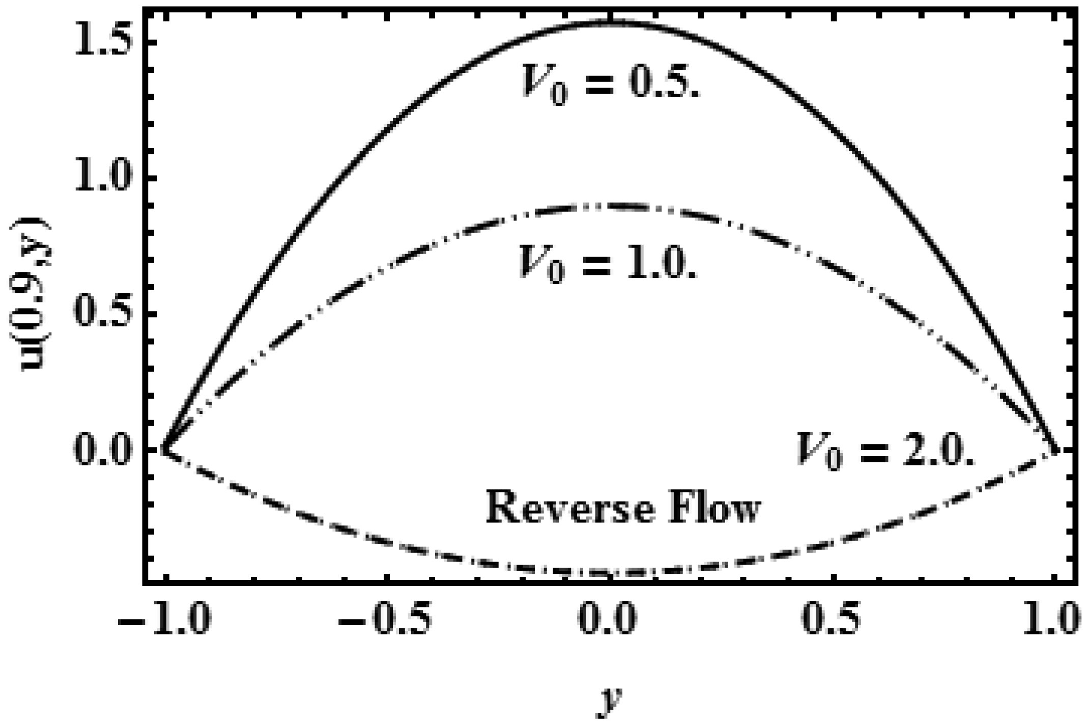
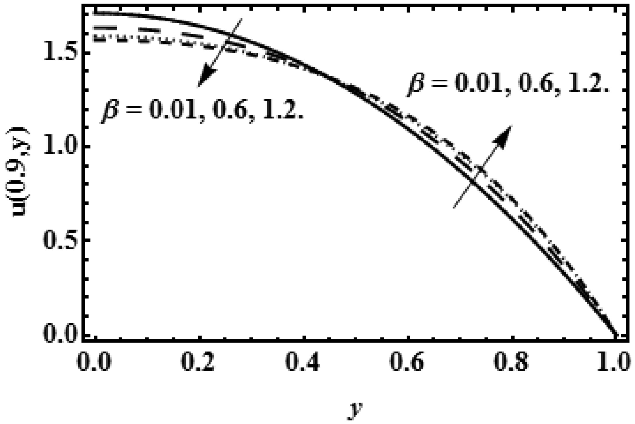
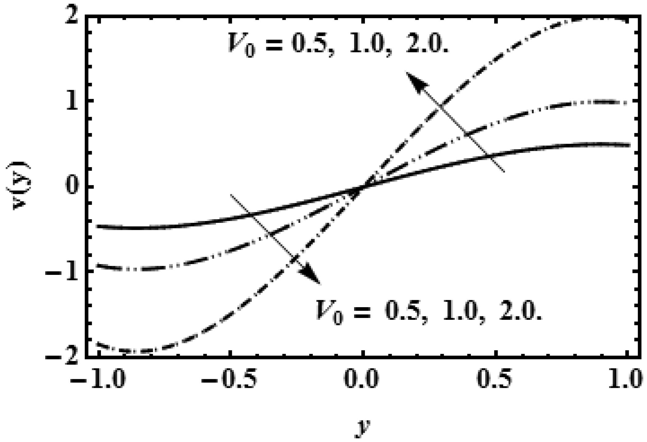
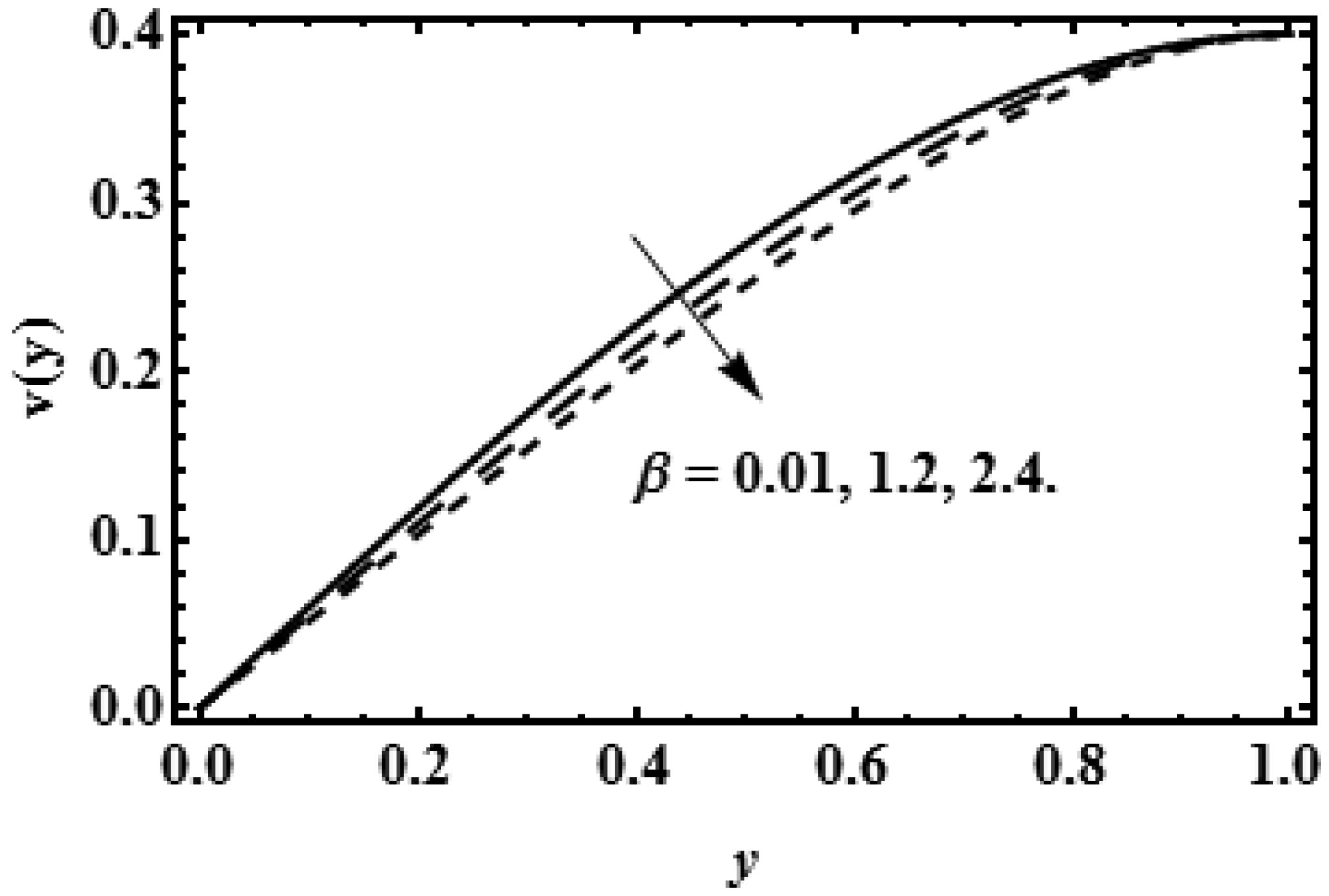
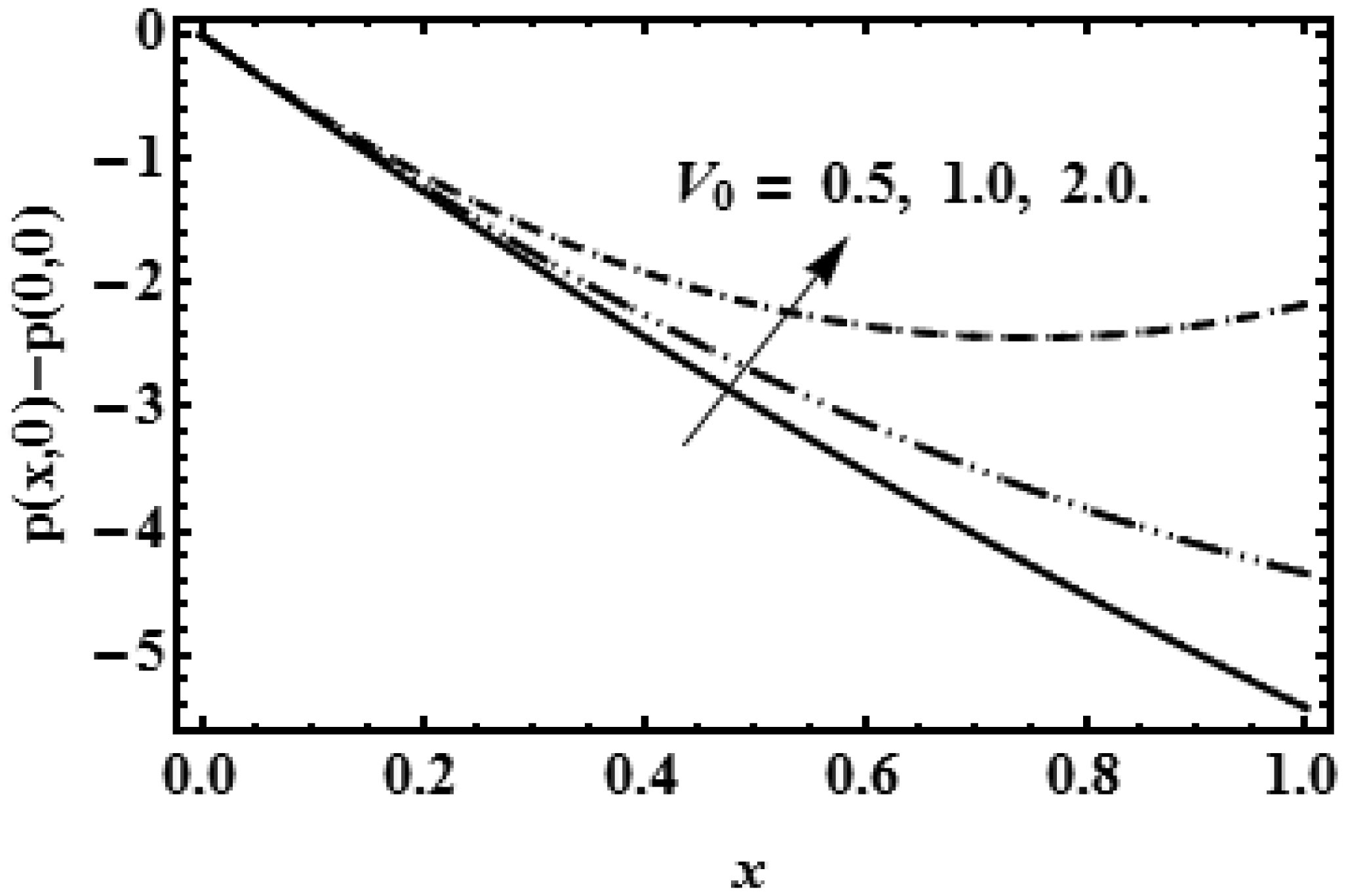
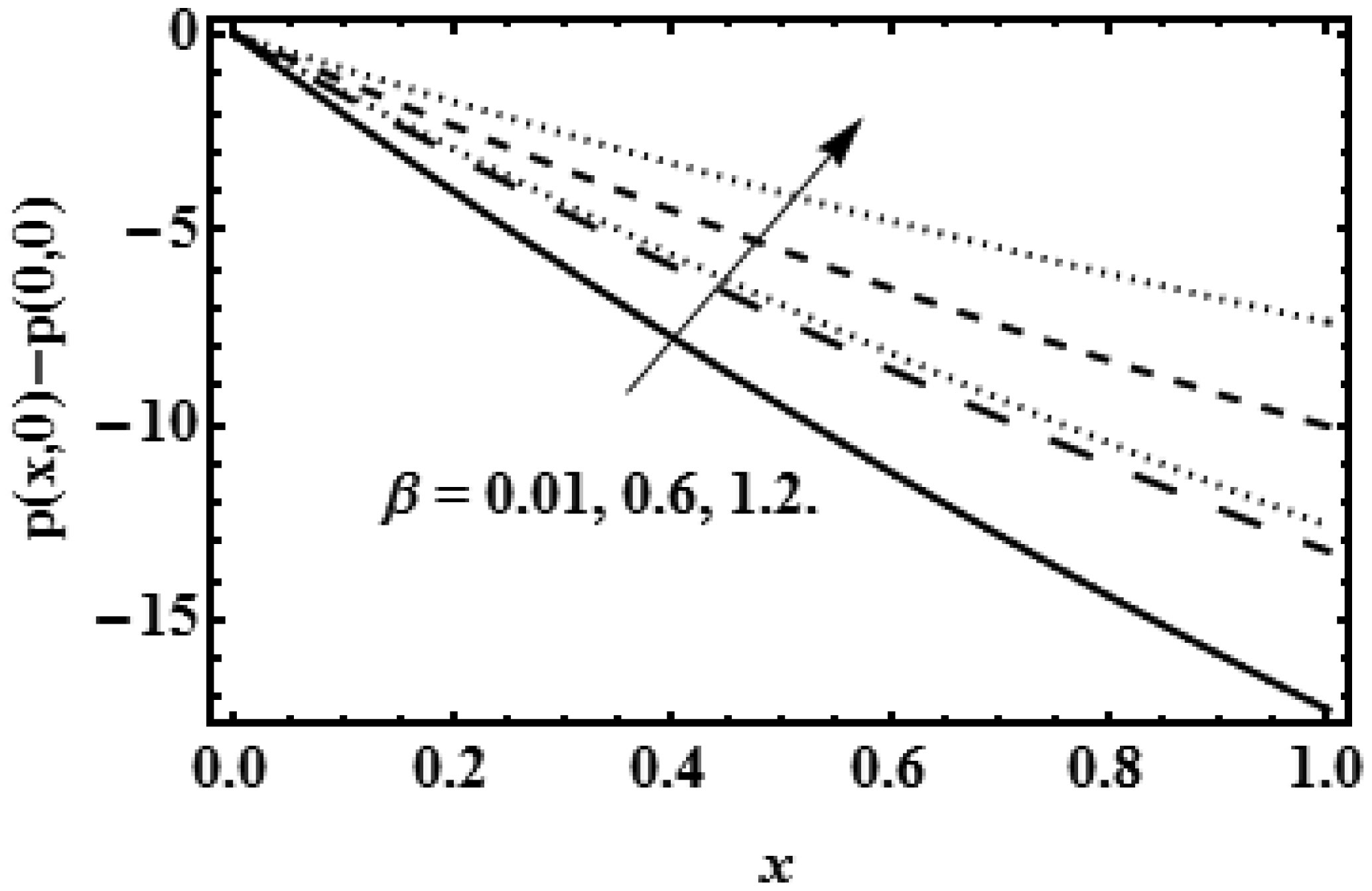
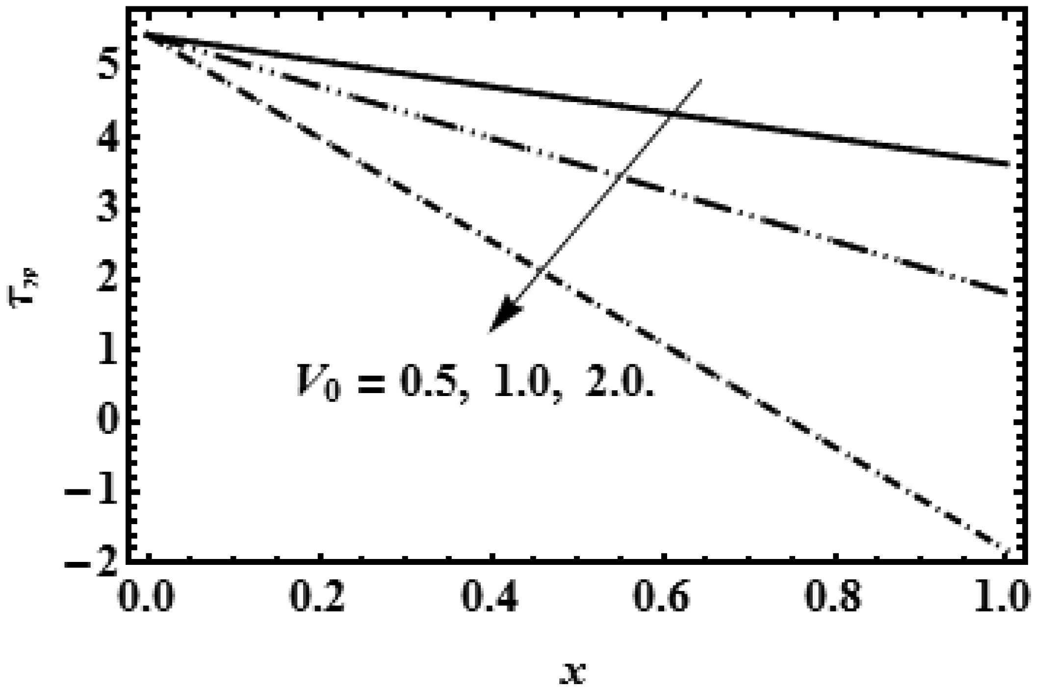
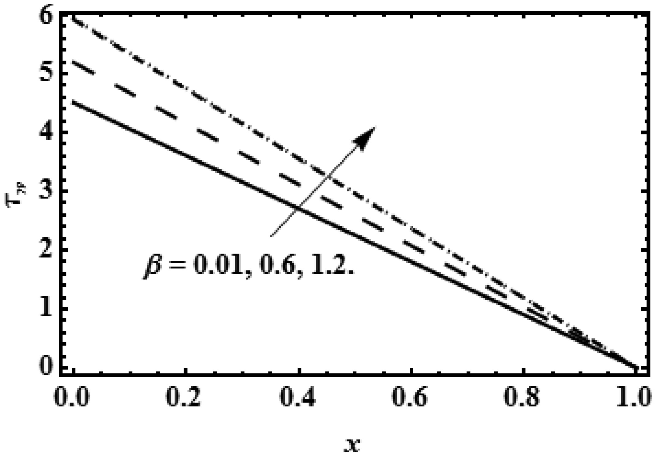
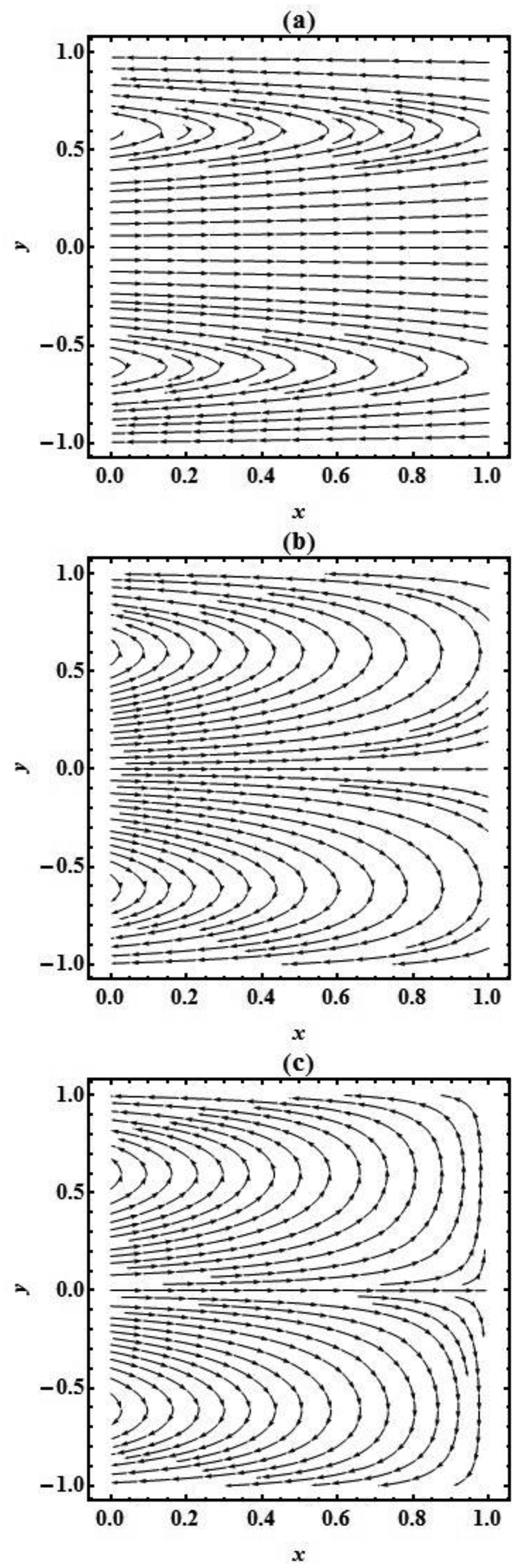
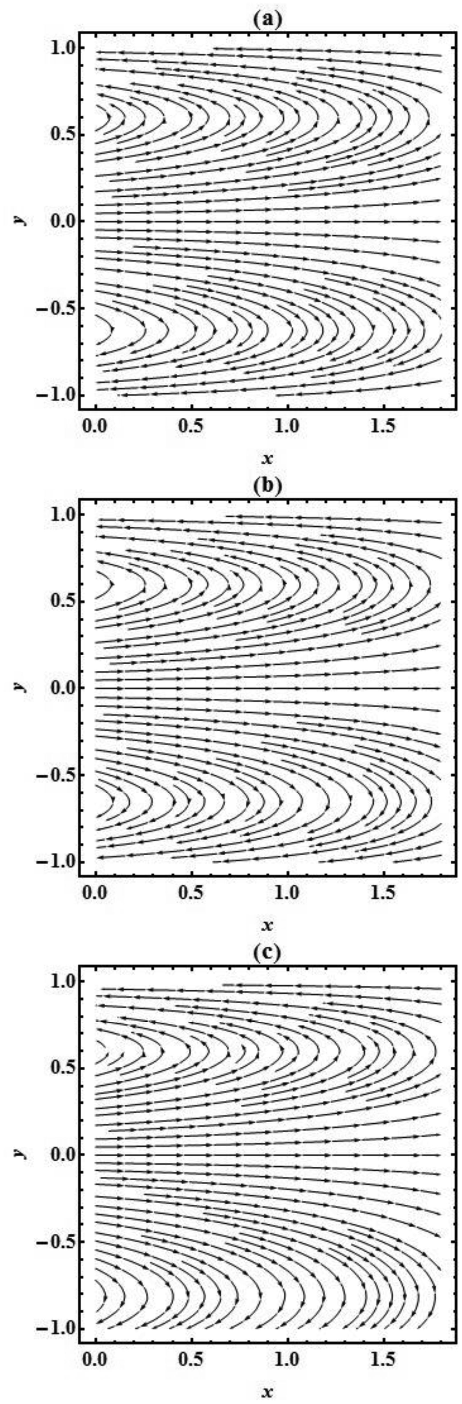
The idea of this study is to present the mathematical model of two-dimensional biofluid flow having variable viscosity along the height of the channel (proximal renal tube of artificial kidney). This research describes that flow resistance is dependent on the height of the channel (proximal renal tube of artificial kidney) which makes the high flow near the centre and slow near the wall. The goal of this research is to provide the formulas to find the flow speed, average pressure, outflow flux and filtration rate of the viscous fluid having variable viscosity. The complex mathematical problem is solved by the Inverse method and results for axial velocity are plotted at the opening, central and departure region of the conduit. The numerical values for constant reabsorption and mean pressure are calculated against the filtration rate for the constant and variable viscosity. The numerical results of pressure rise show that when the viscosity of biofluid varies from centre to the boundary, then high change in pressure is required as compared with the biofluid having constant viscosity along the height of the slit. These mathematical formulas are very useful for the bioengineers to design the portable artificial kidney which works as a mechanical tool to filter the biofluid.

Keywords:

Citation: Khadija Maqbool, Hira Mehboob, Abdul Majeed Siddiqui. Impact of viscosity on creeping viscous fluid flow through a permeable slit: a study for the artificial kidneys[J]. AIMS Biophysics, 2022, 9(4): 308-329. doi: 10.3934/biophy.2022026

Related Papers:

[1]	Abdul M. Siddiqui, Getinet A. Gawo, Khadija Maqbool . On slip of a viscous fluid through proximal renal tubule with linear reabsorption. AIMS Biophysics, 2021, 8(1): 80-102. doi: 10.3934/biophy.2021006
[2]	Boukedjane Mouloud, Bahi Lakhdar . Characterizing pulsatile blood flow in a specific carotid bifurcation: insights into hemodynamics and rheology models. AIMS Biophysics, 2023, 10(3): 281-316. doi: 10.3934/biophy.2023019
[3]	Daniel N. Riahi, Saulo Orizaga . On modeling arterial blood flow with or without solute transport and in presence of atherosclerosis. AIMS Biophysics, 2024, 11(1): 66-84. doi: 10.3934/biophy.2024005
[4]	Mohamed A. Elblbesy, Bothaina A. Kandil . Hemorheological measurements over the shear-thinning regime. In vitro comparative study for hyperglycemia. AIMS Biophysics, 2024, 11(2): 121-129. doi: 10.3934/biophy.2024008
[5]	David Gosselin, Maxime Huet, Myriam Cubizolles, David Rabaud, Naceur Belgacem, Didier Chaussy, Jean Berthier . Viscoelastic capillary flow: the case of whole blood. AIMS Biophysics, 2016, 3(3): 340-357. doi: 10.3934/biophy.2016.3.340
[6]	Bradley Vis, Jonathan J. Powell, Rachel E. Hewitt . Imaging flow cytometry methods for quantitative analysis of label-free crystalline silica particle interactions with immune cells. AIMS Biophysics, 2020, 7(3): 144-166. doi: 10.3934/biophy.2020012
[7]	Wenyuan Xie, Jason Wei Jun Low, Arunmozhiarasi Armugam, Kandiah Jeyaseelan, Yen Wah Tong . Regulation of Aquaporin Z osmotic permeability in ABA tri-block copolymer. AIMS Biophysics, 2015, 2(3): 381-397. doi: 10.3934/biophy.2015.3.381
[8]	Giulia Rigamonti, Marco Guardamagna, Sabina Merlo . Non-contact reflectometric readout of disposable microfluidic devices by near infra-red low-coherence interferometry. AIMS Biophysics, 2016, 3(4): 585-595. doi: 10.3934/biophy.2016.4.585
[9]	Mohamed A. Elblbesy . Impact of erythrocytes properties on blood surface tension. AIMS Biophysics, 2019, 6(2): 39-46. doi: 10.3934/biophy.2019.2.39
[10]	Masoud Jabbary, Hossein Rajabi . High-resolution phantom of a nephron for radiation nephrotoxicity evaluation in biophysical simulations. AIMS Biophysics, 2022, 9(2): 147-160. doi: 10.3934/biophy.2022013

Abstract

1. Introduction

The microstructure of portable artificial kidneys is responsible for the blood filtration and urine formation (mechanical process of biofluid) which acts as a micromachine due to very small size but do the complex process of reabsorption, filtration, excretion and secretion in its different parts. Kidneys contain renal speck and renal tubule; renal speck is further split into glomerulus and Bowman's capsule where blood is filtered through the glomerulus circulates and filtered blood then comes to the renal tubule where reabsorption takes place. Within the nephron, glomerular purification comprises on reflexive movement of blood plasma from glomerulus capillaries to the Bowman's capsule that is easily permeable to H₂O, small solutes like urea, sodium ion, and glucose but not porous to hemoglobin and platelets. The next part of the renal tubule is the proximal convoluted tubule (PCT) where effective and reactive transport take place to reabsorb glucose, sodium chloride, and water from the glomerular filtrate. The current model describes biomechanics of plasma having variable viscosity depending upon the distance from centre to the proximal tube wall that is the main segment of kidneys where constant reabsorption and filtration take place.

Different studies of viscous flow through renal tubule having permeable wall property with constant, linear and nonlinear rate of reabsorption have been discussed. Burgen et. al. [1] introduced a study of viscous flow through kidney with glucose reabsorption and developed mathematical equations for solute reabsorption and used the results to check the high affinity of glucose. The dynamics of biofluid through renal tubule and flow behavior in the presence of constant reabsorption on the wall has been discussed by Macey et. al. [2]. He analysed the viscous flow through infinite cylinder using the Navier Stokes equations with constant and linear reabsorption on the walls of cylinder and noticed the Poiseuille flow for constant reabsorption and for the linear reabsorption the flow lines become flattens instead of curve lines. The dynamical properties of the viscous flow through a permeable tube had been examined by Marshall et. al. [3] and found the exact solution with the help of Navier-Stokes equation for velocity and pressure using the Darcy's law also, the approximate solution for the leakage flux has calculated for the proximal renal tubule. Berkstresser et. al. [4], Tewarson et. al. [5] and Gupta et. al. [6] introduced the numerical and analytic techniques for the solution of mathematical model of viscous flow through renal tubule. Ahmad et al. [7] discussed the exact solution of viscous flow through the renal tube and showed the periodic flow in radial direction of the tube. Muthu et al. [8] presented the finite difference method to find the viscous flow through the cross section of tube with permeable boundary, he found the axial velocity and mean pressure generated by the reabsorption on the wall and flux on the axial direction. Koplik et al. [9], Pozrikidis et al. [10], Kropinski et al. [11] and Haroon et al [12] obtained the results for volume flow rate, glucose reabsorption, velocity and shear stress for Newtonian flow through permeable tube and slit by different methods. They found the slip and no slip effect on the velocity, leakage flux, flow rate and used the resulting formulas to find the reabsorption rate and mean pressure against the fractional reabsorption.

The viscosity of plasma filtered in kidney is not a fixed quantity, but it changes according to the diameter of proximal tubule, also flow resistance in renal tube decreases strongly with reduced diameter of the tube which is less than 0.3mm as mentioned in the study of Gilmer et. al. [13]. The flow resistance of the fluid to be filtered in proximal tube is considerably the case of Poiseuille flow because of pressure gradient which describes that resistance in the flow is low at the centre of tube and high near the tube wall. Few studies have been presented the effect of viscosity on the blood flow through kidney (Lamport et. al. [14],[15], Gaylor et. al. [16] and Omori et. al. [17], Halfenstein et. al. [18], Mukhopadhyay et. al. [19],[20]) but in all these studies only theoretical and experimental data has been used. Recently, Mehboob et. al. [21] presented the effect of variable viscosity and constant reabsorption on the slow viscous flow through narrow straight tubule and found the formulas for the leakage flux, mean pressure drop and flow rate but this problem was formulated in cylindrical coordinate system. There is not a single study available in literature which describes the mathematical formulas of creeping flow having varying viscosity across the height of channel with uniform absorption on the permeable walls of the channel in rectangular coordinate system.

Keeping above studies in mind, it has been assumed that the viscosity is an exponential function of distance from the centre to the boundary and reabsorption on the wall is constant. In this paper to study the effect of exponential type of viscosity for the viscous flow through a kidney, authors have considered the uniform reabsorption on the wall and discussed the problem formulation in section 2, methodology of complex system is included in section 3, mathematical results are presented in fourth section, application of the problem is in section 5, discussion is in section 6 and conclusion is included in section 7.

2. Materials and methods

The present mathematical model suggests that a viscous fluid across a rectangular cross section is flowing under the effect of constant flux applied at the entrance of slit. The -axis locating at the middle of rectangular slit and -axis in the vertical direction of centre line as mentioned in Figure 1, due to symmetric behaviour, the upper half of a rectangular slit has considered to reduce the calculations.

Since the kidney contains the proximal renal tube and movement in this tube is of Poiseuille type Layton et al [22] which requires that axial velocity is highest at the middle of slit that is stated in Eq (7). Since boundaries of renal tubule are permeable and reabsorption takes place through these boundaries at a constant rate which is stated in Eq (8). These hypotheses support to assume that thickness is a decreasing function of distance from base to the boundary, therefore in the current research authors have assumed the Navier-Stokes equation with non-constant viscosity. The current problem of two-dimension, incompressible steady state creeping flow through slit become complicated due to non-constant viscosity.

Figure 1. Schematic diagram of the problem.

DownLoad: Full-Size Img PowerPoint

The suggested model recommends that movement of fluid through a slit satisfy the following flow field.

$V = [u (x, y), v (x, y), 0],$ (1)

where u and v represents horizontal and transverse velocity components.

The fluid flow through the nephron is incompressible i.e density is constant throughout the flow field and satisfy the following continuity equation

$\frac{\partial u}{\partial x} + \frac{\partial v}{\partial y} = 0.$ (2)

The creeping viscous flow across a slit suggests that in the absence of inertia term NSE's with variable viscosity satisfy the following set of equations.

$\frac{\partial p}{\partial x} = \frac{\partial}{\partial x} (2 µ (y) \frac{\partial u}{\partial x}) + \frac{\partial}{\partial y} {µ (y) (\frac{\partial u}{\partial y} + \frac{\partial v}{\partial x})},$ (3)

$\frac{\partial p}{\partial y} = \frac{\partial}{\partial x} {µ (y) (\frac{\partial u}{\partial y} + \frac{\partial v}{\partial x})} + \frac{\partial}{\partial y} (2 µ (y) \frac{\partial v}{\partial y}) .$ (4)

2.1. Exponential viscosity

Case I: $µ (y) = e^{- β y}$

Since the viscosity is a decreasing function of radius of tube which is mentioned in Ref. (Gilmer et al [13]& Tripathi et al [23]) therefore, the variable viscosity in the following form has chosen

$µ (y) = e^{- β y}, β > 0.$ (5)

The assumptions of plasma flow through renal proximal tube and constant reabsorption on the permeable boundary satisfy the following boundary conditions

$\frac{\partial u}{\partial y} = 0, v = 0, a t y = 0,$ (6)

$u = 0, v = V_{0}, a t y = H,$ (7)

$Q_{0} = 2 W \int_{0}^{H} u (0, y) d y .$ (8)

Stream function and velocity profile are associated by the following expressions

$u = \frac{\partial ψ}{\partial y}, v = - \frac{\partial ψ}{\partial x} .$ (9)

The above expressions of stream function and Eqs (3,4) give the following form

$\frac{\partial p}{\partial x} = 2 e^{- β y} \frac{\partial^{3} ψ}{\partial x^{2} \partial y} + \frac{\partial}{\partial y} {e^{- β y} (\frac{\partial^{2} ψ}{\partial y^{2}} - \frac{\partial^{2} ψ}{\partial x^{2}})},$ (10)

$\frac{\partial p}{\partial y} = e^{- β y} \frac{\partial}{\partial x} (\frac{\partial^{2} ψ}{\partial y^{2}} - \frac{\partial^{2} ψ}{\partial x^{2}}) + 2 \frac{\partial}{\partial y} {e^{- β y} (- \frac{\partial^{2} ψ}{\partial x \partial y})} .$ (11)

Eliminating pressure gradient from Eqs (10,11), one can write the following expression.

$\nabla^{4} ψ - β^{2} E^{2} ψ - 2 β \frac{\partial}{\partial y} (\nabla^{2} ψ) = 0,$ (12)

where $\nabla^{2} = \frac{\partial^{2}}{\partial x^{2}} + \frac{\partial^{2}}{\partial y^{2}}$ a and $E^{2} = \frac{\partial^{2}}{\partial x^{2}} - \frac{\partial^{2}}{\partial y^{2}}$ .

Boundary conditions in terms of stream function are given as follows

$\frac{\partial^{2} ψ}{\partial y^{2}} = 0, \frac{\partial ψ}{\partial x} = 0, a t y = 0,$ (13)

$\frac{\partial ψ}{\partial y} = 0, \frac{\partial ψ}{\partial x} = - V_{0}, a t y = H,$ (14)

$ψ (0, 0) = 0, a n d ψ (0, H) = \frac{Q_{0}}{2 W} .$ (15)

The non-dimensional quantities are chosen from Ref. [12]

$\begin{array}{l} x^{*} = \frac{x}{L}, y^{*} = \frac{y}{L}, V_{0}^{*} = \frac{V_{0}}{U_{0}}, ψ^{*} = \frac{ψ}{U_{0} L}, β^{*} = β L, \\ Q_{0}^{*} = \frac{Q_{0}}{U_{0} W L}, τ_{w}^{*} = \frac{τ_{w}}{µ (y) U_{0} / L}, u^{*} = \frac{u}{U_{0}}, v^{*} = \frac{v}{U_{0}}, H^{*} = \frac{H}{L}, \end{array}$ (16)

where U₀ is reference velocity, L is the length of slit, H is the height and W is the width of slit. Nondimensional form of Eqs (12-15) after releasing “*” take the following form

$\nabla^{4} ψ - β^{2} E^{2} ψ - 2 β \frac{\partial}{\partial y} (\nabla^{2} ψ) = 0,$ (17)

$\frac{\partial^{2} ψ}{\partial y^{2}} = 0, \frac{\partial ψ}{\partial x} = 0, a t y = 0,$ (18)

$\frac{\partial ψ}{\partial y} = 0, \frac{\partial ψ}{\partial x} = - V_{0}, a t y = H,$ (19)

$ψ (0, 0) = 0, a n d ψ (0, H) = \frac{Q_{0}}{2 W} .$ (20)

2.1.1. Solution of the problem

To get the solution of problem given in Eqs (17-20), Inverse method [12] is used which requires the following function.

$ψ (x, y) = x R (y) + T (y),$ (21)

where R(y) and T(y) represent unknown functions.

Invoking Eq (21) in Eqs (17-20), one can obtain the following set of equations

$\frac{d^{4} R}{d y^{4}} - 2 β \frac{d^{3} R}{d y^{3}} + β^{2} \frac{d^{2} R}{d y^{2}} = 0,$ (22)

$\frac{d^{4} T}{d y^{4}} - 2 β \frac{d^{3} T}{d y^{3}} + β^{2} \frac{d^{2} T}{d y^{2}} = 0,$ (23)

and boundary conditions are

$R (0) = 0, \frac{d^{2} R (0)}{d y^{2}} = 0,$ (24)

$R (H) = - V_{0}, \frac{d R (H)}{d y} = 0,$ (25)

$T (0) = 0, \frac{d^{2} T (0)}{d y^{2}} = 0,$ (26)

$T (H) = \frac{Q_{0}}{2}, \frac{d T (H)}{d y} = 0.$ (27)

Solving Eqs (22,23) under the boundary conditions (24-27), one can obtained the following expressions for R(y) and T(y)

$(y) = \frac{V_{0} (2 + e^{H β} y β (1 - H β) - e^{y β} (2 - y β))}{- 2 + e^{H β} (2 - H β (2 - H β))},$ (28)

and

$(y) = \frac{Q_{0} (- 2 - e^{H β} y β (1 - H β) + e^{y β} (2 - y β))}{- 4 + e^{H β} (4 - 2 H β (2 - H β))} .$ (29)

Following stream function can be found after using R(y) and T(y) in Eq. (21)

$ψ (x, y) = \frac{(Q_{0} - 2 V_{0} x) (- 2 - e^{H β} y β (1 - H β) + e^{y β} (2 - y β))}{- 4 + e^{H β} (4 - 2 H β (2 - H β))}$ (30)

2.1.2. Velocity distribution

With the aid of above stream function and Eq (9), one can get the next components of velocity

$u (x, y) = \frac{- (Q_{0} - 2 V_{0} x) β (1 - H β - e^{- (H - y) β} (1 - y β))}{4 - 4 e^{- H β} - 2 H β (2 - H β)},$ (31)

and

$v (x, y) = \frac{V_{0} (- 2 - e^{H β} y β (1 - H β) + e^{y β} (2 - y β))}{- 2 + e^{H β} (2 - H β (2 - H β))} .$ (32)

Above equations show that horizontal velocity u(x, y) depends upon x and y, also horizontal velocity is maximum at y = 0 i.e.

$u_{m a x} = \frac{- (Q_{0} - 2 V_{0} x) β (1 - H β - e^{- H β})}{4 - 4 e^{- H β} - 2 H β (2 - H β)},$ (33)

and v(x, y) is maximum at y = H.

$v_{m a x} = V_{0} .$ (34)

Flow rate across the slit can be calculated by the following formula

$Q (x) = 2 \int_{0}^{H} u (x, y) d y,$ (35)

$Q (x) = Q_{0} - 2 V_{0} x,$ (36)

which results from the inlet to the outlet of rectangular cross section.

2.1.3. Pressure

In biological movements pressure performs an important role therefore to find the pressure, Eqs. (9-10) with the help of Eq (31) and Eq (32) are reduced into the following form

$\frac{\partial p}{\partial x} = - β e^{- β y} (x \frac{d^{2} R}{d y^{2}} + \frac{d^{2} T}{d y^{2}}) + e^{- β y} (x \frac{d^{3} R}{d y^{3}} + \frac{d^{3} T}{d y^{3}}),$ (37)

$\frac{\partial p}{\partial y} = - e^{- β y} (\frac{d^{2} R}{d y^{2}} - 2 β \frac{d R}{d y}) .$ (38)

Using R(y) and T(y), Eqs (37,38) take the following form

$\frac{\partial p}{\partial x} = \frac{- (Q_{0} - 2 V_{0} x) β^{3}}{- 4 + e^{H β} (4 - 2 H β (2 - H β))},$ (39)

$\frac{\partial p}{\partial y} = \frac{V_{0} β^{2} (2 e^{- y β} (1 - H β) - e^{- H β} (2 - y β))}{2 - 2 e^{- H β} - H β (2 - H β)} .$ (40)

Integration of above expressions yield the following form

$p (x, y) = \frac{- V_{0} β (4 e^{- y β} (1 - H β) + e^{- H β} y β (4 - y β))}{4 - 4 e^{- H β} - 2 H β (2 - H β)} + f (x),$ (41)

where f(x) i is given by as follows

$f (x) = \frac{- x (Q_{0} - V_{0} x) β^{3}}{- 4 + e^{H β} (4 - 2 H β (2 - H β))} + C,$ (42)

where C is an arbitrary factor. Inserting Eq (42) in Eq (41), we can compose the subsequent form of pressure

$p (x, y) - p (0, 0) = \frac{- β (4 (- 1 + e^{- y β}) V_{0} (1 - H β) + e^{- H β} β (4 V_{0} y + Q_{0} x β - V_{0} (x^{2} + y^{2}) β))}{4 - 4 e^{- H β} - 2 H β (2 - H β)},$ (43)

where p(0, 0) shows pressure at creek of rectangular cross section.

The average pressure drop is defined as follows

$\overset{̅}{p} (x) = \frac{1}{H} \int_{0}^{H} (p (x, y) - p (0, 0)) d y .$ (44)

After inserting value of p(x, y) − p(0, 0) from Eq (43), the above equation takes the following form.

$\overset{̅}{p} (x) = \frac{12 V_{0} {(1 - H β)}^{2} + e^{- H β} (3 H Q_{0} x β^{3} + V_{0} (- 12 - H β (- 12 - 6 H β + (H^{2} + 3 x^{2}) β^{2})))}{12 e^{- H β} - 6 (2 - H β (2 - H β))} .$ (45)

Pressure drops over the length of rectangular cross section is given by the following formula

$Δ \bar{p} (L) = \bar{p} (0) - \bar{p} (L),$ (46)

which reduces to

$Δ \bar{p} (L) = \frac{- e^{- H β} L (- Q_{0} + L V_{0}) β^{3}}{4 - 4 e^{- H β} - 2 H β (2 - H β)} .$ (47)

2.1.4. Wall shear stress

Shear forces are very crucial in the viscous flow with variable viscosity and support to find the resistance on plane which are penned as follows

${τ_{w} |}_{y = H} = - µ (y) {(\frac{\partial u}{\partial y} + \frac{\partial v}{\partial x})}_{y = H},$ (48)

Invoking Eqs (31,32) in above equation, we attained

${τ_{w} |}_{y = H} = \frac{H (Q_{0} - 2 V_{0} x) β^{3}}{4 - 4 e^{- H β} - 2 H β (2 - H β)} .$ (49)

2.1.5. Fractional reabsorption and leakage flux

The ratio of reabsorption to filtration rate can be measured by the following formula

$F A = \frac{Q (0) - Q (L)}{Q (0)} = \frac{2 V_{0} L}{Q_{0}}$ (50)

Leakage flux is given by the following formula

$q (x) = - \frac{d Q (x)}{d x} = 2 V_{0} .$ (51)

2.2. Linear viscosity

Case II: $µ (y) = 1 - β y$

In this case we will take the following viscosity

$µ (y) = 1 - β y, β > 0,$ (52)

After injecting Eq (52) and Eq (9) in Eqs (2,3), we get

$\frac{\partial p}{\partial x} = 2 (1 - β y) \frac{\partial^{3} ψ}{\partial x^{2} \partial y} + \frac{\partial}{\partial y} {(1 - β y) (\frac{\partial^{2} ψ}{\partial y^{2}} - \frac{\partial^{2} ψ}{\partial x^{2}})},$ (53)

$\frac{\partial p}{\partial y} = (1 - β y) \frac{\partial}{\partial x} (\frac{\partial^{2} ψ}{\partial y^{2}} - \frac{\partial^{2} ψ}{\partial x^{2}}) + 2 \frac{\partial}{\partial y} {(1 - β y) (- \frac{\partial^{2} ψ}{\partial x \partial y})} .$ (54)

Reducing pressure gradient from Eqs (53,54), one can obtain the compatibility equation in terms of stream function

$(1 - β y) \nabla^{4} ψ - 2 β \frac{\partial}{\partial y} (\nabla^{2} ψ) = 0,$ (55)

where $\nabla^{2} = \frac{\partial^{2}}{\partial x^{2}} + \frac{\partial^{2}}{\partial y^{2}}$ .

There will be no change in Eq (55) after using non-dimensional quantities given in Eq (16)

2.2.1. Solution of the problem

Substituting Eq (21) into the Eq (55) to get

$(1 - β y) \frac{d^{4} R}{d y^{4}} - 2 β \frac{d^{3} R}{d y^{3}} = 0,$ (56)

$(1 - β y) \frac{d^{4} T}{d y^{4}} - 2 β \frac{d^{3} T}{d y^{3}} = 0.$ (57)

On solving Eqs (56,57) under the boundary conditions (24-27), we get the solution

$R (y) = \frac{V_{0} (- 2 y β \ln (- β + H β^{2}) - 2 \ln (1 - y β) - y β (2 + 2 H β - y β - 2 \ln (- β + y β^{2})))}{- H β (- 2 - H β) + 2 \ln (1 - H β)},$ (58)

and

$T (y) = \frac{Q_{0} (2 y β \ln (- β + H β^{2}) + 2 \ln (1 - y β) - y β (- 2 - 2 H β + y β + 2 \ln (- β + y β^{2})))}{- 2 H β (- 2 - H β) + 4 \ln (1 - H β)},$ (59)

Invoking R(y) and T(y) into Eq. (21) to get the following stream function

$ψ (x, y) = \frac{(2 y β \ln (- β + H β^{2}) + 2 \ln (1 - y β) - y β (- 2 - 2 H β + y β + 2 \ln (- β + y β^{2})))}{2 H β (2 + H β) + 4 \ln (1 - H β)} (Q_{0} - 2 V_{0} x) .$ (60)

2.2.2. Velocity field

With the aid of Eq (9) and Eq (60), flow field in axial and vertical direction are found as follows

$u (x, y) = \frac{- (Q_{0} - 2 V_{0} x) β (- (H - y) β - \ln (- β + H β^{2}) + \ln (- β + y β^{2}))}{H β (2 + H β) + 2 ln (1 - H β)},$ (61)

and

$v (x, y) = \frac{V_{0} (2 y β \ln (- β + H β^{2}) + 2 \ln (1 - y β) - y β (- 2 - 2 H β + y β + 2 \ln (- β + y β^{2})))}{H β (2 + H β) + 2 ln (1 - H β)} .$ (62)

Horizontal velocity is maximum at y = 0.

$u_{m a x} = \frac{- (Q_{0} - 2 V_{0} x) β (- H β + ln (- β) - \ln (- β + H β^{2}))}{H β (2 + H β) + 2 ln (1 - H β)},$ (63)

and v(x, y) is maximum at y = H.

$v_{m a x} = V_{0} .$ (64)

Flow rate within the four-sided slit is attained by using Eq (61) in Eq (35).

$Q (x) = Q_{0} - 2 V_{0} x .$ (65)

2.2.3. Pressure distribution

To find pressure, Eqs (53,54) can be composed in following manner

$\frac{\partial p}{\partial x} = - β (x \frac{d^{2} R}{d y^{2}} + \frac{d^{2} T}{d y^{2}}) + (1 - β y) (x \frac{d^{3} R}{d y^{3}} + \frac{d^{3} T}{d y^{3}}),$ (66)

$\frac{\partial p}{\partial y} = - (1 - β y) \frac{d^{2} R}{d y^{2}} + 2 β \frac{d R}{d y} .$ (67)

By using Eqs (58,59) in Eqs (66,67) to get

$\frac{\partial p}{\partial x} = \frac{(Q_{0} - 2 V_{0} x) β^{3}}{H β (2 + H β) + 2 \ln (1 - H β)},$ (68)

$\frac{\partial p}{\partial y} = \frac{2 V_{0} β^{2} (- 2 H β + 3 y β - 2 \ln (- β + H β^{2}) + 2 \ln (- β + y β^{2}))}{H β (2 + H β) + 2 \ln (1 - H β)} .$ (69)

Integrating Eq (69) yields

$p (x, y) = \frac{(Q_{0} - V_{0} x) x β^{3}}{H β (2 + H β) + 2 \ln (1 - H β)} + H (y),$ (70)

where H(y) is given by as follows

$H (y) = \frac{- V_{0} β (4 y β \ln (- β + H β^{2}) + 4 \ln (1 - y β) - y β (- 4 - 4 H β + 3 y β + 4 \ln (- β + y β^{2})))}{H β (2 + H β) + 2 \ln (1 - H β)} + C,$ (71)

where C is an arbitrary factor. Using Eq (71) in Eq (70), we can write the subsequent form of pressure

$p (x, y) - p (0, 0) = - β (- β (Q_{0} x β + V_{0} (- x^{2} β + y (- 4 - 4 H β + 3 y β))) + 4 V_{0} (\ln (1 - y β) - y β (- \ln (- β + H β^{2}) + \ln (- β + y β^{2})))) / H β (2 + H β) + 2 ln (1 - H β),$ (72)

where p(0, 0) shows the pressure at entrance of the slit.

Mean pressure drop can be find by substituting the value of p(x, y) − p(0, 0) in Eq (44) as follows

$\overset{̅}{p} (x) = V_{0} (\frac{1}{H} - 2 β) + \frac{(H^{2} V_{0} + x (Q_{0} - V_{0} x)) β^{3}}{H β (2 + H β) + 2 \ln (1 - H β)} .$ (73)

To get the pressure drop over the length L, invoke the values of p(0) and p(L) in Eq (47).

$Δ \bar{p} (L) = - \frac{L (Q_{0} - L V_{0}) β^{3}}{H β (2 + H β) + 2 ln (1 - H β)} .$ (74)

2.2.4. Wall shear stress

Invoking Eqs (61,62) in Eq (48) to attain wall shear stress

${τ_{w} |}_{y = H} = - \frac{H (Q_{0} - 2 V_{0} x) β^{3}}{(1 - H β) (H β (2 + H β) + 2 \ln (1 - H β))} .$ (75)

3. Constant viscosity

Case III: If we apply the limit β → 0 on Eq 31, 32 and 43 and solving the resulting expressions by the L' Hospital rule, one can attain the results of constant viscosity µ which are same as mentioned in Ref. [12].

$ψ (x, y) = \frac{1}{2} (\frac{Q_{0}}{2} - V_{0} x) \frac{y}{H} (3 - {(\frac{y}{H})}^{2}),$ (76)

$u (x, y) = \frac{3 (Q_{0} - 2 V_{0} x)}{4 H} (1 - {(\frac{y}{H})}^{2}),$ (77)

$v (x, y) = \frac{V_{0}}{2} \frac{y}{H} (3 - {(\frac{y}{H})}^{2}),$ (78)

$p (x, y) - p (0, 0) = - \frac{3 µ (Q_{0} - V_{0} x) x}{2 H^{3}} - \frac{3 µ V_{0} y^{2}}{2 H^{3}} .$ (79)

4. Application to kidneys flow

We have utilized biological data of mammalian kidneys to find the values of V₀ and Δp in artificial renal tubule which is assumed to be the permeable channel. In this study length of artificial renal tubule (slit) is chosen to be L = 0.12cm and height of slit has considered as H = 0.0005cm, average viscosity µ = 6.9×10⁻³dynsec/cm², Q₀ = 1.25×10⁻⁴cm³/sec, β = 2.5×10⁻³/cm and W = 0.1 cm (as $H ≪ W$ ) from Zhang et al [24]. Table 1 shows the calculated values of mean pressure and reabsorption rate for the constant and variable viscosity. As cited in Refs. (Mehboob et. al. [21], Layton et al [22], Korkmaz et al [25], Herranz et al [26] and Tortora et al [27] in usual conditions glomerulus pressure is assumed to be about $45 m m H g (59995.07433675 d y n / c m^{2})$ which is above the average pressure than that observed in tubes elsewhere in the body. It has stated in Table 1 the reducing values of reabsorption rate causes to lower the fractional reabsorption, but the average pressure drop in the renal tubule enhances with the falling values of reabsorption rate, also the assumption of variable viscosity indicate that average pressure drop is elevated as matched with the case of constant viscosity.

The results of this study are beneficial to measure the change in pressure compared to the fractional reabsorption because the viscosity of the liquid decay near the boundary which is the consequence of lubricating nature of permeable wall. The numerical values given in table 1 indicate that the various rate of reabsorption requires the different mean pressure which may be supportive for the patients of nephrotic disorder. The present data from table 1 also support the person that how much intake of fluid is needed to generate the mean pressure next to the filtration rate which has examined by the blood CP and urine test.

Table 1. Fractional reabsorption, reabsorption rate of fluid and pressure variation for persistent (constant) viscosity and variable viscosity in a renal tubule.

Viscosity	FA	90%	80%	70%	60%
	V₀cm/sec	4.7×10⁻³	4.2×10⁻³	3.6×10⁻³	3.1×10⁻³
Constant	Δp(0.12)dyn/cm²	1212.19	2404.51	3835.3	5027.62
Variable	Δp(0.12)dyn/cm²	6460.62	7025.69	7703.78	8268.84

| Show Table

DownLoad: CSV

5. Results

Figure 2. Effect of V₀ at entrance region (x = 0.1).

DownLoad: Full-Size Img PowerPoint

Figure 3. Effect of β at entrance region (x = 0.1).

DownLoad: Full-Size Img PowerPoint

Figure 4. Effect of V₀ at middle region (x = 0.5).

DownLoad: Full-Size Img PowerPoint

Figure 5. Effect of β at middle region (x = 0.5).

DownLoad: Full-Size Img PowerPoint

Figure 6. Effect of V₀ at exit region (x = 0.9).

DownLoad: Full-Size Img PowerPoint

Figure 7. Effect of β at exit region (x = 0.9).

DownLoad: Full-Size Img PowerPoint

Figure 8. Effect of V₀ in the tranverse direction of flow.

DownLoad: Full-Size Img PowerPoint

Figure 9. Effect of β in the transverse direction of flow.

DownLoad: Full-Size Img PowerPoint

Figure 10. Effect of V₀ on pressure difference.

DownLoad: Full-Size Img PowerPoint

Figure 11. Effect of β on pressure difference.

DownLoad: Full-Size Img PowerPoint

Figure 12. Effect of V₀ on wall shear stress.

DownLoad: Full-Size Img PowerPoint

Figure 13. Effect of β on wall shear stress.

DownLoad: Full-Size Img PowerPoint

Figure 14. (a) V₀ = 0.4, (b) V₀ = 1.2, (c) V₀ = 1.5.

DownLoad: Full-Size Img PowerPoint

Figure 15. (a) β = 0.1, (b) β = 0.2, (c) β = 0.65.

DownLoad: Full-Size Img PowerPoint

6. Discussion

In this research the mathematical results of flow speed, flow pattern, pressure and shearing force are presented by the graphs which are plotted in software Mathematica under the effect of different values of reabsorption velocity V₀ and viscosity parameter β at x = 0.1, x = 0.5, x = 0.9, which are entry, central and leaving points of the rectangular cross section respectively.

Figures (2), (4) and (6) show the decaying effect of reabsorption rate V₀ on axial velocity at the points x = 0.1, 0.5, 0.9 on the slit and observe that decay is swifter near the center region (x = 0.5) but near the departure region (x = 0.9) back flow has been examined. It has been noted that near the centre of slit drift is highest due to change in pressure and near the borders of slit (y = h) the fluid movement become motionless due to deposition of the particles (reabsorption V₀).

Figures (3), (5) and (7) explain the decelerating impact of viscosity parameter β on axial rate near the center of the slit at the points x = 0.1, 0.5, 0.9 of the slit. The axial flow rises away from the centre (y = h) and decays near the centre line (y = 0) due to the growing values of viscosity parameter β, because resistance at the boundary wall (y = h) makes the motionless flow at the boundary but the resistive forces become stronger near the centre of slit (y = 0) due to pressure gradient $\frac{d p}{d x}$ which helps to make the decreasing effect on axial velocity.

Figure 8 illustrates the variation of reabsorption rate V₀ at the vertical direction of flow field, which displays the symmetry about the centre line (y = 0). The presence of reabsorption V₀ indicates the growing effect on the transverse flow near the permeable membrane of renal tube. Decaying effect of viscosity parameter β on the vertical flow is displayed through the Figure 9, it is observed that the resistive force retards the movement of the fluid molecules in vertical direction.

The pressure p plays a vital role for the flow of viscous fluid, therefore graphical results for pressure p are displayed in Figure 10 and Figure 11. The decreasing effect of reabsorption velocity V₀ on pressure difference is displayed in Figure 10 which shows that presence of reabsorption V₀ on the membrane require the low change in pressure for the viscous flow through permeable channel and the pressure at the entrance x = 0.1 is high as compared with the other region x = 0.9 of the slit. Figure 11 indicates that rising values of β help to reduce the pressure difference from entry point x = 0.1 to the centre line y = 0, which is evidenced that decreasing viscosity β help to reduce the pressure for the viscous fluid flow.

When the fluid is in contact with the surface then wall shear stress is an important phenomenon on the boundary surface. The variation in wall shear stress against V₀ is described in Figure 12 which shows the reduction in the shear stress on the wall with the mounting values of reabsorption V₀. The constant reabsorption V₀ on the wall helps to reduce the shearing forces on the permeable wall, which indicates that flow across the tube move easily without the large load. The rising values of parameter β results to improve the shearing forces on the wall because the growing values of β increases the resistance near the boundary wall which requires the high load for the fluid flow near the boundary.

The pattern of the flow field can be observed by the streamlines which are plotted in Figure 14 (a-c) and Figure 15 (a-c). It is examined that addition in reabsorption velocity V₀ triggers the number of lines which indicates that the fluid is becoming thin in the presence of reabsorption V₀, but the number of streamlines reduces with the mounting values of viscosity parameter β which indicates that fluid is going to be thin, and it contains more resistance for the fluid flow.

7. Conclusions

This research presents the mathematical modelling of plasma flow through the renal tube, the two-dimensional slit in rectangular coordinate is considered in the analogy of proximal renal tube and viscous fluid is assumed as a plasma with variable viscosity from centre line to the boundary surface due to reabsorption on the permeable wall. The complex mathematical model is solved by the inverse method and exact expression for flow speed, load, shear force and filtration are calculated. The application of the present study is presented with the numerical data present in the literature. The special cases for the linear and constant reabsorption are also obtained and observed that results of constant reabsorptions match with the existing results (Haroon et al. [12]) which validates the current research. The impact of reabsorption and viscosity parameter on the physical quantities of the flow field are observed through graphs. The numerical results of mean pressure and constant reabsorption against filtration rate show that constant viscosity of the plasma in slit requires less amount of average pressure but the biofluid having variable viscosity along the slit requires high average pressure for the fluid flow.

Acknowledgments

We appreciate the reviewer's insightful feedback, which helped us refine this study.

Conflict of interest

No potential conflicts of interest were disclosed by the author(s) with regard to the research, writing, or publication of this paper.

Author contributions

Khadija Maqbool supervised and conceived the idea. Hira Mehboob wrote the manuscript and revising it critically. A. M. Siddiqui helped in graphical depiction and final approval of the version to be published. Concerns about the precision or reliability of any aspect of the work will be duly investigated and addressed by corresponding author.

References

[1]	Burgen ASV (1956) A theoretical treatment of glucose reabsorption in the kidney. Can J Biochem Phys 34: 466-474. https://doi.org/10.1139/y56-048
[2]	Macey RI (1965) Hydrodynamics in the renal tubule. Bull Math Biophys 27: 117-124. https://doi.org/10.1007/BF02498766
[3]	Marshall EA, Trowbridge EA (1974) Flow of a Newtonian fluid through a permeable tube: the application to the proximal renal tubule. Bull Math Biol 36: 457-476. https://doi.org/10.1007/BF02463260
[4]	Berkstresser BK, El-Asfouri S, McConnell JR, et al. (1979) Identification techniques for the renal function. Math Biosci 44: 157-165. https://doi.org/10.1016/0025-5564(79)90078-6
[5]	Tewarson RP (1981) On the use of Simpson's rule in renal models. Math Biosci 55: 1-5. https://doi.org/10.1016/0025-5564(81)90009-2
[6]	Gupta S, Tewarson RP (1983) On accurate solution of renal models. Math Biosci 65: 199-207. https://doi.org/10.1016/0025-5564(83)90061-5
[7]	Ahmad S, Ahmad N (2011) On flow through renal tubule in case of periodic radial velocity component. Int J Emerg Multidiscip Fluid Res 3: 201-208. https://doi.org/10.1260/1756-8315.3.4.201
[8]	Muthu P, Berhane T (2011) Flow of Newtonian fluid in non-uniform tubes with application to renal flow: a numerical study. Adv Appl Math Mech 3: 633-648. https://doi.org/10.4208/aamm.10-m1064
[9]	Koplik J (1982) Creeping flow in two-dimensional networks. J Fluid Mech 119: 219-247. https://doi.org/10.1017/S0022112082001323
[10]	Pozrikidis C (1987) Creeping flow in two-dimensional channels. J Fluid Mech 180: 495-514. https://doi.org/10.1017/S0022112087001927
[11]	Kropinski MCA (2001) An efficient numerical method for studying interfacial motion in two-dimensional creeping flows. J Comput Phys 171: 479-508. https://doi.org/10.1006/jcph.2001.6787
[12]	Haroon T, Siddiqui AM, Shahzad A (2016) Creeping flow of viscous fluid through a proximal tubule with uniform reabsorption: a mathematical study. Appl Math Sci 10: 795-807. https://doi.org/10.12988/ams.2016.512739
[13]	Gilmer GG, Deshpande VG, Chou CL, et al. (2018) Flow resistance along the rat renal tubule. Am J Physiol Renal Physiol 315: F1398-F1405. https://doi.org/10.1152/ajprenal.00219.2018
[14]	Lamport H (1943) Improvements in calculation of renal resistance to blood flow. charts for osmotic pressure and viscosity of blood. J Clin Invest 22: 461-470. https://doi.org/10.1172/JCI101416
[15]	Lamport H (1942) The effects on renal resistance to blood flow of renin, angiotonin, pitressin and atropine, hypertension, and toxemia of pregnancy. J Clin Invest 21: 685-695. https://doi.org/10.1172/JCI101345
[16]	Gaylor JDS (1973) Thin film blood flow in rectangular channels with application to artificial kidney haemodynamics. J Biomech 6: 241-251. https://doi.org/10.1016/0021-9290(73)90046-8
[17]	Omori T, Wada S, Tsubota KI, et al. (2006) Multi-scale simulation of blood flow with the dynamical behavior of elastic red blood cells. J Biomech 39: S649. http://dx.doi.org/10.1016%2FS0021-9290(06)85706-4
[18]	Helfenstein C, Gennisson JL, Tanter M, et al. (2015) Effects of pressure on the shear modulus, mass and thickness of the perfused porcine kidney. J Biomech 48: 30-37. https://doi: 10.1016/j.jbiomech.2014.11.011
[19]	Mukhopadhyay S, Mukhopadhyay A (2021) Hydrodynamic instability and wave formation of a viscous film flowing down a slippery inclined substrate: effect of odd-viscosity. Eur J Mech-B/Fluids 89: 161-170. https://doi.org/10.1016/j.euromechflu.2021.05.013
[20]	Mukhopadhyay S, Cellier N, Usha R, et al. (2022) Falling film on an anisotropic porous medium. J Fluid Mech 947: A26. https://doi.org/10.1017/jfm.2022.634
[21]	Mehboob H, Maqbool K, Siddiqui AM, et al. (2021) Mathematical analysis of viscosity and reabsorption on urine flow through a straight narrow tube. Biomed Eng-Appl Basis Commun 33: 2150039. https://doi.org/10.4015/S1016237221500393
[22]	Layton AT, Layton HE (2019) A computational model of epithelial solute and water transport along a human nephron. PLoS Comput Biol 15: e1006108. https://doi.org/10.1371/journal.pcbi.1006108
[23]	Tripathi D, Pandey SK, Siddiqui A, et al. (2014) Non-steady peristaltic propulsion with exponential variable viscosity: a study of transport through the digestive system. Computer Methods in Biomechanics and Biomedical Engineering : 591-603. https://doi.org/10.1080/10255842.2012.703660
[24]	Zhang SY, Mahler GJ (2021) Modelling renal filtration and reabsorption processes in a human glomerulus and proximal tubule microphysiological system. Micromachines 12: 983. https://doi.org/10.3390/mi12080983
[25]	Korkmaz I, Rogg B (2006) Simulation of urine flow through the male lower urinary tract. J Biomech 39: S389-S390. http://dx.doi.org/10.1016%2FS0021-9290(06)84574-4
[26]	Herranz B, Álvarez MD, Pérez-Jiménez J (2018) Association of plasma and urine viscosity with cardiometabolic risk factors and oxidative status. a pilot study in subjects with abdominal obesity. PloS One 13: e0204075. https://doi.org/10.1371/journal.pone.0204075
[27]	Tortora GJ, Derrickson BH (2018) Principles of Anatomy and Physiology.John Wiley and Sons.

This article has been cited by:

José H Valladares Pérez, Roberto Márquez Islas, Celia Sánchez Pérez, Augusto García Valenzuela, Measurement of resistivity of biofluids in the presence of an electrical double layer, 2025, 36, 0957-0233, 025113, 10.1088/1361-6501/adaa94

Reader Comments

Your name:*

Email:*
© 2022 the Author(s), licensee AIMS Press. This is an open access article distributed under the terms of the Creative Commons Attribution License (http://creativecommons.org/licenses/by/4.0)

通讯作者: 陈斌, bchen63@163.com

1.
沈阳化工大学材料科学与工程学院沈阳 110142

AIMS Biophysics

1.1 2.4

Metrics

Article views(1578) PDF downloads(84) Cited by(1)

Preview PDF

Download XML

Export Citation

Article outline

Show full outline

Figures and Tables

Figures(15) / Tables(1)

AIMS Biophysics

Impact of viscosity on creeping viscous fluid flow through a permeable slit: a study for the artificial kidneys

Related Papers:

Abstract

1. Introduction

2. Materials and methods

2.1. Exponential viscosity

2.1.1. Solution of the problem

2.1.2. Velocity distribution

2.1.3. Pressure

2.1.4. Wall shear stress

2.1.5. Fractional reabsorption and leakage flux

2.2. Linear viscosity

2.2.1. Solution of the problem

2.2.2. Velocity field

2.2.3. Pressure distribution

2.2.4. Wall shear stress

3. Constant viscosity

4. Application to kidneys flow

5. Results

6. Discussion

7. Conclusions

References

This article has been cited by:

Reader Comments

通讯作者: 陈斌, bchen63@163.com

Metrics

Figures and Tables

Other Articles By Authors

Catalog

AIMS Biophysics

Impact of viscosity on creeping viscous fluid flow through a permeable slit: a study for the artificial kidneys

Related Papers:

Abstract

1. Introduction

2. Materials and methods

2.1. Exponential viscosity

2.1.1. Solution of the problem

2.1.2. Velocity distribution

2.1.3. Pressure

2.1.4. Wall shear stress

2.1.5. Fractional reabsorption and leakage flux

2.2. Linear viscosity

2.2.1. Solution of the problem

2.2.2. Velocity field

2.2.3. Pressure distribution

2.2.4. Wall shear stress

3. Constant viscosity

4. Application to kidneys flow

5. Results

6. Discussion

7. Conclusions

References

This article has been cited by:

Reader Comments

通讯作者: 陈斌, bchen63@163.com

Metrics

Figures and Tables

Other Articles By Authors

Related pages

Tools

Export File

Citation

Format

Content

Catalog