Low energy electron beam (e-beam) has the ability to decontaminate or reduce bioburden and enhance the food product's safety with minimal quality loss. The current study aimed to evaluate the efficacy of e-beam on natural microbiota and quality changes in black peppercorns. The black pepper was exposed to e-beam at doses from 6–18 kGy. The microbial quality, physicochemical attributes, total phenolic compounds, and antioxidant activity were evaluated. Results demonstrated the microbial population in black pepper decreased with increasing e-beam treatment doses. Significant inactivation of Total Plate Count (TPC), yeasts, and molds were observed at dose 6 kGy by 2.3, 0.7, and 1.3 log CFU g−1, respectively, while at 18 kGy the reduction level was 6, 2.9, and 4.4 log CFU g−1, respectively. Similarly, 18 kGy of e-beam yielded a reduction of 3.3 and 3.1 log CFU g−1 of Salmonella Typhimurium and coliform bacteria, respectively. A significant difference (p < 0.05) was noted between doses 12, 15, and 18 kGy on Bacillus cereus and Clostridium perfringens in black pepper. During e-beam doses, the values L*, a* and b* of black peppercorn were not noticeably altered up to 18 kGy dose. No significant (p > 0.05) difference in moisture, volatile oil, and piperine content upon (6–18 kGy) treatments in comparison to the control. A slight difference in the bioactive compound, retaining > 90% of total phenolic compounds and antioxidant activity. Results revealed that e-beam doses ≥ 18 kGy were influential for inactivating natural microbes and foodborne pathogens without compromising the physicochemical properties and antioxidant activity of black peppercorns.
Citation: Abdul Basit M. Gaba, Mohamed A. Hassan, Ashraf A. Abd El-Tawab, Mohamed A. Abdelmonem, Mohamed K. Morsy. Impact of low energy electron beam on black pepper (Piper nigrum L.) microbial reduction, quality parameters, and antioxidant activity[J]. AIMS Agriculture and Food, 2022, 7(3): 737-749. doi: 10.3934/agrfood.2022045
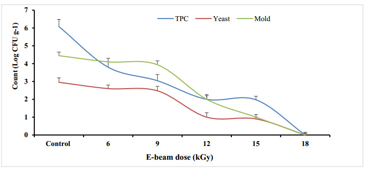
Low energy electron beam (e-beam) has the ability to decontaminate or reduce bioburden and enhance the food product's safety with minimal quality loss. The current study aimed to evaluate the efficacy of e-beam on natural microbiota and quality changes in black peppercorns. The black pepper was exposed to e-beam at doses from 6–18 kGy. The microbial quality, physicochemical attributes, total phenolic compounds, and antioxidant activity were evaluated. Results demonstrated the microbial population in black pepper decreased with increasing e-beam treatment doses. Significant inactivation of Total Plate Count (TPC), yeasts, and molds were observed at dose 6 kGy by 2.3, 0.7, and 1.3 log CFU g−1, respectively, while at 18 kGy the reduction level was 6, 2.9, and 4.4 log CFU g−1, respectively. Similarly, 18 kGy of e-beam yielded a reduction of 3.3 and 3.1 log CFU g−1 of Salmonella Typhimurium and coliform bacteria, respectively. A significant difference (p < 0.05) was noted between doses 12, 15, and 18 kGy on Bacillus cereus and Clostridium perfringens in black pepper. During e-beam doses, the values L*, a* and b* of black peppercorn were not noticeably altered up to 18 kGy dose. No significant (p > 0.05) difference in moisture, volatile oil, and piperine content upon (6–18 kGy) treatments in comparison to the control. A slight difference in the bioactive compound, retaining > 90% of total phenolic compounds and antioxidant activity. Results revealed that e-beam doses ≥ 18 kGy were influential for inactivating natural microbes and foodborne pathogens without compromising the physicochemical properties and antioxidant activity of black peppercorns.

| [1] |
Jiang TA (2019) Health benefits of culinary herbs and spices. J AOAC Int 102: 395–411. https://doi.org/10.5740/jaoacint.18-0418 doi: 10.5740/jaoacint.18-0418

|
| [2] |
Székács A, Wilkinson MG, Mader A, et al. (2018) Environmental and food safety of spices and herbs along global food chains. Food Control 83: 1–6. https://doi.org/10.1016/j.foodcont.2017.06.033 doi: 10.1016/j.foodcont.2017.06.033
|
| [3] | Sultan NA (2019) The consistency of export and agricultural policies in Egypt.[Master's Thesis, the American University in Cairo]. AUC Knowledge Fountain. https://fount.aucegypt.edu/etds/849 |
| [4] |
Nguyen L, Duong LT, Mentreddy RS (2019) The US import demand for spices and herbs by differentiated sources. J. Appl Res Med Aromat Plants 12: 13–20. https://doi.org/10.1016/j.jarmap.2018.12.001 doi: 10.1016/j.jarmap.2018.12.001
|
| [5] |
Man A, Mare A, Toma F, et al. (2016) Health threats from contamination of spices commercialized in romania: Risks of fungal and bacterial infections. Endocr Metab Immune Disord—Drug Targets (Formerly Current Drug Targets-Immune, Endocrine & Metabolic Disorders) 16: 197–204. https://doi.org/10.2174/1871530316666160823145817 doi: 10.2174/1871530316666160823145817
|
| [6] |
Nur F, Libra UK, Rowsan P, et al. (2018) Assessment of bacterial contamination of dried herbs and spices collected from street markets in Dhaka. Bangladesh J Pharmacol 21: 96–100. https://doi.org/10.3329/bpj.v21i2.37919 doi: 10.3329/bpj.v21i2.37919
|
| [7] | Nielsen K (2016) Spicy Food as Cause of Death—Coincidence and Necessity in Metaphysics E 2–3. |
| [8] |
Lv J, Qi L, Yu C, et al. (2015) Consumption of spicy foods and total and cause specific mortality: Population based cohort study. BMJ 351: h3942. https://doi.org/10.1136/bmj.h3942 doi: 10.1136/bmj.h3942
|
| [9] |
Stojanović-Radić Z, Pejčić M, Dimitrijević M, et al. (2019) Piperine—A major principle of black pepper: A review of its bioactivity and studies. Appl Sci 9: 4270. https://doi.org/10.3390/app9204270 doi: 10.3390/app9204270
|
| [10] |
Gülçin İ (2005) The antioxidant and radical scavenging activities of black pepper (Piper nigrum) seeds. Int J Food Sci Nutr 56: 491–499. https://doi.org/10.1080/09637480500450248 doi: 10.1080/09637480500450248
|
| [11] | Sharma N, Sharma T, Choudhary J (2021) Antimicrobial activity of some herbal feed additives. Pharma Innov 10: 392–394. |
| [12] |
Banerjee M, Sarkar PK (2003) Microbiological quality of some retail spices in India. Food Res Int 36: 469–474. https://doi.org/10.1016/S0963-9969(02)00194-1 doi: 10.1016/S0963-9969(02)00194-1
|
| [13] | CDC (2010) Investigation update: Multistate outbreak of human Salmonella Montevideo infections. Centers for Disease Control and Prevention Atlanta, GA. |
| [14] |
Van Doren JM, Neil KP, Parish M, et al. (2013) Foodborne illness outbreaks from microbial contaminants in spices, 1973–2010. Food Microbiol 36: 456–464. https://doi.org/10.1016/j.fm.2013.04.014 doi: 10.1016/j.fm.2013.04.014
|
| [15] |
Scallan E, Hoekstra RM, Angulo FJ, et al. (2011) Foodborne illness acquired in the United States—Major pathogens. Emerg Infect Dis 17: 7–15. https://doi.org/10.3201/eid1701.P11101 doi: 10.3201/eid1701.P11101
|
| [16] | CDC (Centers for Disease Control and Prevention) (2011) Vital signs: Incidence and trends of infection with pathogens transmitted commonly through foode foodborne diseases active surveillance network. 10 U.S. sites, 1996–2010. Morb Mortal Wkly Rep 60: 749–755. |
| [17] |
Bakobie N, Addae AS, Duwiejuah AB, et al. (2017) Microbial profile of common spices and spice blends used in tamale, Ghana. Int J Food Cont 4: 1–5. https://doi.org/10.1186/s40550-017-0055-9 doi: 10.1186/s40550-017-0055-9
|
| [18] |
Golden CE, Berrang ME, Kerr WL, et al. (2019) Slow-release chlorine dioxide gas treatment as a means to reduce Salmonella contamination on spices. Innovative Food Sci & Emerging Technol 52: 256–261. https://doi.org/10.1016/j.ifset.2019.01.003 doi: 10.1016/j.ifset.2019.01.003
|
| [19] | Caver CB (2016) Recovery of Salmonella from Steam and Ethylene Oxide-Treated Spices Using Supplemented Agar with Overlay. Masters Theses, Virginia Tech. http://hdl.handle.net/10919/81456 |
| [20] |
Jinot J, Fritz JM, Vulimiri SV, et al. (2018) Carcinogenicity of ethylene oxide: key findings and scientific issues. Toxicol Mech Methods 28: 386–396. https://doi.org/10.1080/15376516.2017.1414343 doi: 10.1080/15376516.2017.1414343
|
| [21] | Peter K (2006) Handbook of herbs and spices: Woodhead publishing. |
| [22] | Bagdatlioglu N, Orman S (2010) The effect of steam sterilization on antioxidant activities of sage, oregano and basil. Ital J Food Sci 22: 343. |
| [23] |
Gryczka U, Kameya H, Kimura K, et al. (2020) Efficacy of low energy electron beam on microbial decontamination of spices. Radiat. Phys Chem 170: 1–5. https://doi.org/10.1016/j.radphyschem.2019.108662 doi: 10.1016/j.radphyschem.2019.108662
|
| [24] |
Ehlermann DA (2016) The early history of food irradiation. Radiat Phys Chem 129: 10–12. https://doi.org/10.1016/j.radphyschem.2016.07.024 doi: 10.1016/j.radphyschem.2016.07.024
|
| [25] |
Roberts PB (2016) Food irradiation: Standards, regulations and world-wide trade. Radiat Phys Chem 129: 30–34. https://doi.org/10.1016/j.radphyschem.2016.06.005 doi: 10.1016/j.radphyschem.2016.06.005
|
| [26] | Wilkinson VM (1997) Food irradiation: A reference guide: CRC Press. |
| [27] | Molins RA (2001) Food irradiation: Principles and applications: John Wiley & Sons. |
| [28] | Demirci A, Ngadi MO (2012) Microbial decontamination in the food industry: Novel methods and applications: Woodhead Publishing. |
| [29] |
Fertey J, Bayer L, Grunwald T, et al. (2016) Pathogens inactivated by low-energy-electron irradiation maintain antigenic properties and induce protective immune responses. Viruses 8: 319. https://doi.org/10.3390/v8110319 doi: 10.3390/v8110319
|
| [30] |
Zhang Y, Moeller R, Tran S, et al. (2018) Geobacillus and Bacillus spore inactivation by low energy electron beam technology: resistance and influencing factors. Front Microbiol 9: 2720. https://doi.org/10.3389/fmicb.2018.0272 doi: 10.3389/fmicb.2018.0272
|
| [31] |
Baek M-e, Ameer K, Jo Y, et al. (2019) Microbial assessment of medicinal herbs (Cnidii Rhizoma and Alismatis Rhizoma), effects of electron beam irradiation and detection characteristics. Food Sci Biotechnol 29: 705–715. https://doi.org/10.1007/s10068-019-00701-w doi: 10.1007/s10068-019-00701-w
|
| [32] |
Gryczka U, Migdał W, Bułka S (2018) The effectiveness of the microbiological radiation decontamination process of agricultural products with the use of low energy electron beam. Radiat Phys Chem 143: 59–62. https://doi.org/10.1016/j.radphyschem.2017.09.020 doi: 10.1016/j.radphyschem.2017.09.020
|
| [33] |
Zhang H, Zhang Y, Chambers Ⅳ E, et al. (2020) Electron beam irradiation on Fuzhuan brick-tea: Effects on sensory quality and chemical compositions. Radiat Phys Chem 170: 108597. https://doi.org/10.1016/j.radphyschem.2019.108597 doi: 10.1016/j.radphyschem.2019.108597
|
| [34] |
Woldemariam HW, Kießling M, Emire SA, et al. (2021) Influence of electron beam treatment on naturally contaminated red pepper (Capsicum annuum L.) powder: Kinetics of microbial inactivation and physicochemical quality changes. Innovative Food Sci & Emerging Technol 67: 102588. https://doi.org/10.1016/j.ifset.2020.102588 doi: 10.1016/j.ifset.2020.102588
|
| [35] |
Helt-Hansen J, Miller A, Sharpe P, et al. (2010) Dμ—A new concept in industrial low-energy electron dosimetry. Radiat Phys Chem 79: 66–74. https://doi.org/10.1016/j.radphyschem.2009.09.002 doi: 10.1016/j.radphyschem.2009.09.002
|
| [36] | Yousef AE, Carlstrom C (2003) Food microbiology: A laboratory manual: John Wiley & Sons. |
| [37] |
Liu X, Ardo S, Bunning M, et al. (2007) Total phenolic content and DPPH radical scavenging activity of lettuce (Lactuca sativa L.) grown in Colorado. LWT-Food Sci Technol 40: 552–557. https://doi.org/10.1016/j.lwt.2005.09.007 doi: 10.1016/j.lwt.2005.09.007
|
| [38] | Ebrahimzadeh MA, Nabavi SM, Nabavi SF, et al. (2010) Antioxidant and free radical scavenging activity of H. officinalis L. var. angustifolius, V. odorata, B. hyrcana and C. speciosum. Pak J Pharm Sci 23: 29–34. |
| [39] | Berns RS (2019) Billmeyer and Saltzman's principles of color technology: John Wiley & Sons. |
| [40] |
Hajimahmoodi M, Faramarzi MA, Mohammadi N, et al. (2010) Evaluation of antioxidant properties and total phenolic contents of some strains of microalgae. J Appl Phycol 22: 43–50. https://doi.org/10.1007/s10811-009-9424-y doi: 10.1007/s10811-009-9424-y
|
| [41] | AOAC (2016) Association of Official Analytical Chemists. Official Methods of Analysis. (20th Ed.) Maryland, USA. 2016. |
| [42] | Steel RG, Torrie JH (1986) Principles and procedures of statistics: A biometrical approach: McGraw-Hill New York, NY, USA. |
| [43] |
Esmaeili S, Barzegar M, Sahari MA, et al. (2018) Effect of gamma irradiation under various atmospheres of packaging on the microbial and physicochemical properties of turmeric powder. Radiat Phys Chem 148: 60–67. https://doi.org/10.1016/j.radphyschem.2018.02.028 doi: 10.1016/j.radphyschem.2018.02.028
|
| [44] |
Byun K-H, Cho M-J, Park S-Y, et al. (2019) Effects of gamma ray, electron beam, and X-ray on the reduction of Aspergillus flavus on red pepper powder (Capsicum annuum L.) and gochujang (red pepper paste). Food Sci Technol Inter 25: 649–658. https://doi.org/10.1177/1082013219857019 doi: 10.1177/1082013219857019
|
| [45] |
Gryczka U, Madureira J, Verde SC, et al. (2021) Determination of pepper microbial contamination for low energy e-beam irradiation. Food Microbiol 98: 103782. https://doi.org/10.1016/j.fm.2021.103782 doi: 10.1016/j.fm.2021.103782
|
| [46] |
Rico CW, Kim G-R, Ahn J-J, et al. (2010) The comparative effect of steaming and irradiation on the physicochemical and microbiological properties of dried red pepper (Capsicum annum L.). Food Chem 119: 1012–1016. https://doi.org/10.1016/j.foodchem.2009.08.005 doi: 10.1016/j.foodchem.2009.08.005
|
| [47] | Barkai-Golan R, Follett PA (2017) Irradiation for quality improvement, microbial safety and phytosanitation of fresh produce: Academic Press. |
| [48] |
Pauli G, Tarantino L (1995) FDA regulatory aspects of food irradiation. J Food Prot 58: 209–212. https://doi.org/10.4315/0362-028X-58.2.209 doi: 10.4315/0362-028X-58.2.209
|
| [49] |
Lee E-J, Ameer K, Kim G-R, et al. (2018) Effects of approved dose of e-beam irradiation on microbiological and physicochemical qualities of dried laver products and detection of their irradiation status. Food Sci Biotechnol 27: 233–240. https://doi.org/10.1007/s10068-017-0194-z doi: 10.1007/s10068-017-0194-z
|
| [50] |
Kundu D, Gill A, Lui C, et al. (2014) Use of low dose e-beam irradiation to reduce E. coli O157: H7, non-O157 (VTEC) E. coli and Salmonella viability on meat surfaces. Meat Sci 96: 413–418. https://doi.org/10.1016/j.meatsci.2013.07.034 doi: 10.1016/j.meatsci.2013.07.034
|
| [51] |
Nieto-Sandoval JM, Almela L, Fernandez-Lopez JA, et al. (2000) Effect of electron beam irradiation on color and microbial bioburden of red paprika. J Food Prot 63: 633–637. https://doi.org/10.4315/0362-028X-63.5.633 doi: 10.4315/0362-028X-63.5.633
|
| [52] |
Duncan SE, Moberg K, Amin KN, et al. (2017) Processes to preserve spice and herb quality and sensory integrity during pathogen inactivation. J Food Sci 82: 1208–1215. https://doi.org/10.1111/1750-3841.13702 doi: 10.1111/1750-3841.13702
|
| [53] |
Kotilainen H, Meneses N, Laaksonen O, et al. (2021) Effects of low-energy electron beam (LEEB) treatment on physicochemical attributes of black pepper and coriander. Innovative Food Sci & Emerging Technol 2021: 79–100. https://doi.org/10.1016/B978-0-08-100596-5.23013-8 doi: 10.1016/B978-0-08-100596-5.23013-8
|
| [54] | Sádecká J, Kolek E, Petka J, et al. (2005) Impact of gamma-irradiation on microbial decontamination and organoleptic quality of oregano (Origanum vulgare L.). Proceedings of Euro Food Chem XIII, Hamburg 2005: 590–594. |
| [55] |
Rahman M, Islam M, Das KC, et al. (2021) Effect of gamma radiation on microbial load, physico-chemical and sensory characteristics of common spices for storage. J Food Sci Technol 58: 3579–3588. https://doi.org/10.1007/s13197-021-05087-4 doi: 10.1007/s13197-021-05087-4
|
| [56] |
Song W-J, Sung H-J, Kim S-Y, et al. (2014) Inactivation of Escherichia coli O157: H7 and Salmonella Typhimurium in black pepper and red pepper by gamma irradiation. Int J Food Microbiol 172: 125–129. https://doi.org/10.1016/j.ijfoodmicro.2013.11.017 doi: 10.1016/j.ijfoodmicro.2013.11.017
|
| [57] |
Bambirra MLA, Junqueira RG, Glória MBA (2002) Influence of post harvest processing conditions on yield and quality of ground turmeric (Curcuma longa L.). Braz Arch Biol Technol 45: 423–429. https://doi.org/10.1590/S1516-89132002000600004 doi: 10.1590/S1516-89132002000600004
|
| [58] |
Koseki PM, Villavicencio ALC, Brito MS, et al. (2002) Effects of irradiation in medicinal and eatable herbs. Radiat Phys Chem 63: 681–684. https://doi.org/10.1016/S0969-806X(01)00658-2 doi: 10.1016/S0969-806X(01)00658-2
|
| [59] | Jamshidi M, Barzegar M, Sahari M (2014) Effect of gamma and microwave irradiation on antioxidant and antimicrobial activities of Cinnamomum zeylanicum and Echinacea purpurea. Inter Food Res J 21: 1289–1296. |
| [60] |
Variyar PS (1998) Effect of gamma‐irradiation on the phenolic acids of some Indian spices. Int J Food Sci & Technol 33: 533–537. https://doi.org/10.1046/j.1365-2621.1998.00219.x doi: 10.1046/j.1365-2621.1998.00219.x
|
| [61] |
Sajilata M, Singhal R (2006) Effect of irradiation and storage on the antioxidative activity of cashew nuts. Radiat Phys Chem 75: 297–300. https://doi.org/10.1016/j.radphyschem.2005.07.004 doi: 10.1016/j.radphyschem.2005.07.004
|
| [62] |
Fernandes Â, Barreira JC, Antonio AL, et al. (2016) Extended use of gamma irradiation in wild mushrooms conservation: Validation of 2 kGy dose to preserve their chemical characteristics. LWT-Food Sci Technol 67: 99–105. https://doi.org/10.1016/j.lwt.2015.11.038 doi: 10.1016/j.lwt.2015.11.038
|


Figures(4) / Tables(1)

Abdul Basit M. Gaba, Mohamed A. Hassan, Ashraf A. Abd El-Tawab, Mohamed A. Abdelmonem, Mohamed K. Morsy. Impact of low energy electron beam on black pepper (Piper nigrum L.) microbial reduction, quality parameters, and antioxidant activity[J]. AIMS Agriculture and Food, 2022, 7(3): 737-749. doi: 10.3934/agrfood.2022045


 DownLoad: