A nonlocal population model for the invasion of Canada goldenrod

Jian Fang; Na Li; Chenhe Xu; Jian Fang; Na Li; Chenhe Xu

doi:10.3934/mbe.2022462

Mathematical Biosciences and Engineering

2022, Volume 19, Issue 10: 9915-9937. doi: 10.3934/mbe.2022462

Previous Article Next Article

Research article Special Issues

A nonlocal population model for the invasion of Canada goldenrod

Jian Fang ^{1
,
,},
Na Li ¹,
Chenhe Xu ²

1.
School of Mathematics, Harbin Institute of Technology, Harbin, Heilongjiang 150001, China
2.
Department of Applied Mathematics, Hong Kong Polytechnic University, Hung Hom, Kowloon Hong Kong, China

^*In memory of Professor Stephen A. Gourley.
Academic Editor: Feng-Bin Wang

Received: 09 November 2021 Revised: 26 June 2022 Accepted: 05 July 2022 Published: 12 July 2022

A mathematical model for the population invasion of Canada goldenrod is proposed, with two reproductive modes, yearly periodic time delay and spatially nonlocal response caused by the influence of wind on the seeds. Under suitable conditions, we obtain the existence of the rightward and leftward invasion speeds and their coincidence with the minimal speeds of time periodic traveling waves. Furthermore, the invasion speeds are finite if the dispersal kernel of seeds is exponentially bounded and infinite if dispersal kernel is exponentially unbounded.
- Canada goldenrod,
- periodic delay,
- nonlocal dispersal,
- propagation dynamics
Citation: Jian Fang, Na Li, Chenhe Xu. A nonlocal population model for the invasion of Canada goldenrod[J]. Mathematical Biosciences and Engineering, 2022, 19(10): 9915-9937. doi: 10.3934/mbe.2022462

Related Papers:

Abstract

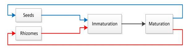
A mathematical model for the population invasion of Canada goldenrod is proposed, with two reproductive modes, yearly periodic time delay and spatially nonlocal response caused by the influence of wind on the seeds. Under suitable conditions, we obtain the existence of the rightward and leftward invasion speeds and their coincidence with the minimal speeds of time periodic traveling waves. Furthermore, the invasion speeds are finite if the dispersal kernel of seeds is exponentially bounded and infinite if dispersal kernel is exponentially unbounded.

References

[1]	H. Lu, H. Ruan, G. Tang, Y. Cai, Z. Gu, J. Wang, Evaluation of harmfulness and utility on Canada Goldenrod (Solidago canadensis), J. Shanghai Jiaotong Univ. (agriculture science), 24 (2006), 402–406.
[2]	M. Čapek, The possibility of biological control of imported weeds of the genus Solidago L. in Europe, Acta Inst. For. Zvolensis, 2 (1971), 429–441.
[3]	P. A. Werner, R. S. Gross, I. K. Bradbury, The biology of canadian weeds.: 45. Solidago canadensis L., Can. J. Plant Sci., 60 (1980), 1393–1409. https://doi.org/10.4141/cjps80-194 doi: 10.4141/cjps80-194
[4]	G. Shen, H. Yao, L. Guan, Z. Qian, Y. Ao, Distribution and Infestation of Canada goldenrod in Shanghai Suburbs and its chemical control, Acta Agric. Shanghai, 21 (2005), 1–4.
[5]	H. Huang, S. Guo, G. Chen, Reproductive biology in an invasive plant Solidago canadensis, Front. Biol. China, 2 (2007), 196–204. https://doi.org/10.1007/s11515-007-0030-6 doi: 10.1007/s11515-007-0030-6
[6]	S. A. Gourley, N. F. Britton, Instability of travelling wave solutions of a population model with nonlocal effects, IMA J. Appl. Math., 51 (1993), 299–310. https://doi.org/10.1093/imamat/51.3.299 doi: 10.1093/imamat/51.3.299
[7]	J. Al-Omari, S. A. Gourley, Monotone travelling fronts in an age-structured reaction-diffusion model of a single species, J. Math. Biol., 45 (2002), 294–312. https://doi.org/10.1007/s002850200159 doi: 10.1007/s002850200159
[8]	S. A. Gourley, Y. Kuang, Wavefronts and global stability in a time-delayed population model with stage structure, Proc. R. Soc. Lond. Ser. A, 459 (2003), 1563–1579. https://doi.org/10.1098/rspa.2002.1094 doi: 10.1098/rspa.2002.1094
[9]	S. A. Gourley, S. Ruan, Convergence and travelling fronts in functional differential equations with nonlocal terms: a competition model, SIAM J. Math. Anal., 35 (2003), 806–822. https://doi.org/10.1137/S003614100139991 doi: 10.1137/S003614100139991
[10]	S. A. Gourley, R. Liu, J. Wu, Spatiotemporal patterns of disease spread: Interaction of physiological structure, spatial movements, disease progression and human intervention, Lect. Notes Math., 1936 (2008), 165–208. https://doi.org/10.1007/978-3-540-78273-5_4 doi: 10.1007/978-3-540-78273-5_4
[11]	S. A. Gourley, J. Wu, Delayed nonlocal diffusive systems in biological invasion and disease spread, Fields Inst. Commun., 48 (2006), 137–200. https://doi.org/10.1090/fic/048/06 doi: 10.1090/fic/048/06
[12]	S. A. Gourley, X. Zou, A mathematical model for the control and eradication of a wood boring beetle infestation, SIAM J. Appl. Math., 68 (2008), 1665–1687. https://doi.org/10.1137/100818510 https://doi.org/10.1137/060674387
[13]	B. L. Phillips, G. P. Brown, J. K. Webb, S. Richard, Invasion and the evolution of speed in toads, Nature, 439 (2006), 803. https://doi.org/10.1038/439803a doi: 10.1038/439803a
[14]	J. S. Clark, Why trees migrate so fast: confronting theory with dispersal biology and the paleorecord, Amer. Nat., 152 (1998), 204–224. https://doi.org/10.1086/286162 doi: 10.1086/286162
[15]	K. Lisa, M. Jeffrey, T. Rebecca, F. Lutscher, Modelling the dynamics of invasion and control of competing green crab genotypes, Theor. Ecol., 7 (2014), 391–406. https://doi.org/10.1007/s12080-014-0226-8 doi: 10.1007/s12080-014-0226-8
[16]	J. Medlock, M. Kot, Spreading disease: integro-differential equations old and new, Math. Biosci., 184 (2003), 201–222. https://doi.org/10.1016/S0025-5564(03)00041-5 doi: 10.1016/S0025-5564(03)00041-5
[17]	Z. Szymańska, C. M. Rodrigo, M. Lchowicz, M. A. J. Chaplain, Mathematical modelling of cancer invasion of tissue: the role and effect of nonlocal interactions, Math. Models Methods Appl. Sci., 19 (2009), 257–281. https://doi.org/10.1142/S0218202509003425 doi: 10.1142/S0218202509003425
[18]	J. Garnier, Accelerating solutions in integro-differential equations, SIAM J. Math. Anal., 43 (2011), 1955–1974. https://doi.org/10.1137/10080693X doi: 10.1137/10080693X
[19]	Y. Pan, J. Fang, J. Wei, Seasonal influence on stage-structured invasive species with yearly generation, SIAM J. Appl. Math., 78 (2018), 1842–1862. https://doi.org/10.1137/17M1145690 doi: 10.1137/17M1145690
[20]	Y. Pan, Y. Su, J. Wei, Accelerating propagation in a recursive system arising from seasonal population models with nonlocal dispersal, J. Differ. Equ., 267 (2019), 150–179. https://doi.org/10.1016/j.jde.2019.01.009 doi: 10.1016/j.jde.2019.01.009
[21]	J. A. Metz, O. Diekmann, The dynamics of physiologically structured populations, Lect. Notes Biomath., 68 (1986). https://doi.org/10.1007/978-3-662-13159-6 doi: 10.1007/978-3-662-13159-6
[22]	X. Liang, X-Q. Zhao, Asymptotic speeds of spread and traveling waves for monotone semiflows with applications, Comm. Pure Appl. Math., 60 (2007), 1–40. https://doi.org/10.1002/cpa.20154 https://doi.org/10.1002/cpa.20221
[23]	H. F. Weinberger, Long-time behavior of a class of biological models, SIAM J. Math. Anal., 13 (1982), 353–396. https://doi.org/10.1137/0513028 doi: 10.1137/0513028
[24]	H. F. Weinberger, X-Q. Zhao, An extension of the formula for spreading speeds, Math. Biosci. Eng., 7 (2010), 187–194. https://doi.org/10.3934/mbe.2010.7.187 doi: 10.3934/mbe.2010.7.187
[25]	J. Fang, X-Q. Zhao, Traveling waves for monotone semiflows with weak compactness, SIAM J. Math. Anal., 46 (2014), 3678–3704. https://doi.org/10.1137/140953939 doi: 10.1137/140953939
[26]	Y. Lou, X.-Q. Zhao, A theoretical approach to understanding population dynamics with seasonal developmental durations, J. Nonlinear Sci., 27 (2017), 573–603. https://doi.org/10.1007/s00332-016-9344-3 doi: 10.1007/s00332-016-9344-3
[27]	J. Fang, J. Wei, X-Q. Zhao, Spatial dynamics of a nonlocal and time-delayed reaction-diffusion system, J. Differ. Equ., 245 (2008), 2749–2770. https://doi.org/10.1016/j.jde.2008.09.001 doi: 10.1016/j.jde.2008.09.001

Reader Comments

Your name:*

Email:*
© 2022 the Author(s), licensee AIMS Press. This is an open access article distributed under the terms of the Creative Commons Attribution License (http://creativecommons.org/licenses/by/4.0)