


The paper is concerned with development of an accurate and effective positivity-preserving high-order compact difference method for solving the Keller-Segel chemotaxis model, which is a kind of nonlinear parabolic-parabolic system in mathematical biology. Firstly, a stiffly-stable five-step fourth-order fully implicit compact difference scheme is proposed. The new scheme not only has fourth-order accuracy in the spatial direction, but also has fourth-order accuracy in the temporal direction, and the computational strategy for the nonlinear chemotaxis term is provided. Then, a positivity-preserving numerical algorithm is presented, which ensures the non-negativity of cell density at all time without accuracy loss. And a time advancement algorithm is established. Finally, the proposed method is applied to the numerical simulation for chemotaxis phenomena, and the accuracy, stability and positivity-preserving of the new scheme are validated with several numerical examples.
Citation: Lin Zhang, Yongbin Ge, Zhi Wang. Positivity-preserving high-order compact difference method for the Keller-Segel chemotaxis model[J]. Mathematical Biosciences and Engineering, 2022, 19(7): 6764-6794. doi: 10.3934/mbe.2022319
| [1] | Fangyuan Chen, Rong Yuan . Dynamic behavior of swine influenza transmission during the breed-slaughter process. Mathematical Biosciences and Engineering, 2020, 17(5): 5849-5863. doi: 10.3934/mbe.2020312 |
| [2] | Zi Sang, Zhipeng Qiu, Xiefei Yan, Yun Zou . Assessing the effect of non-pharmaceutical interventions on containing an emerging disease. Mathematical Biosciences and Engineering, 2012, 9(1): 147-164. doi: 10.3934/mbe.2012.9.147 |
| [3] | Rocio Caja Rivera, Shakir Bilal, Edwin Michael . The relation between host competence and vector-feeding preference in a multi-host model: Chagas and Cutaneous Leishmaniasis. Mathematical Biosciences and Engineering, 2020, 17(5): 5561-5583. doi: 10.3934/mbe.2020299 |
| [4] | Yinggao Zhou, Jianhong Wu, Min Wu . Optimal isolation strategies of emerging infectious diseases with limited resources. Mathematical Biosciences and Engineering, 2013, 10(5&6): 1691-1701. doi: 10.3934/mbe.2013.10.1691 |
| [5] | Robert Stephen Cantrell, Chris Cosner, Yuan Lou . Evolution of dispersal and the ideal free distribution. Mathematical Biosciences and Engineering, 2010, 7(1): 17-36. doi: 10.3934/mbe.2010.7.17 |
| [6] | Fangyuan Chen, Rong Yuan . Reconsideration of the plague transmission in perspective of multi-host zoonotic disease model with interspecific interaction. Mathematical Biosciences and Engineering, 2020, 17(5): 4422-4442. doi: 10.3934/mbe.2020244 |
| [7] | Kuang-Hui Lin, Yuan Lou, Chih-Wen Shih, Tze-Hung Tsai . Global dynamics for two-species competition in patchy environment. Mathematical Biosciences and Engineering, 2014, 11(4): 947-970. doi: 10.3934/mbe.2014.11.947 |
| [8] | Ricardo López-Ruiz, Danièle Fournier-Prunaret . Complex Behavior in a Discrete Coupled Logistic Model for the Symbiotic Interaction of Two Species. Mathematical Biosciences and Engineering, 2004, 1(2): 307-324. doi: 10.3934/mbe.2004.1.307 |
| [9] | S.A. Gourley, Yang Kuang . Two-Species Competition with High Dispersal: The Winning Strategy. Mathematical Biosciences and Engineering, 2005, 2(2): 345-362. doi: 10.3934/mbe.2005.2.345 |
| [10] | Christian Cortés García . Bifurcations in discontinuous mathematical models with control strategy for a species. Mathematical Biosciences and Engineering, 2022, 19(2): 1536-1558. doi: 10.3934/mbe.2022071 |
The paper is concerned with development of an accurate and effective positivity-preserving high-order compact difference method for solving the Keller-Segel chemotaxis model, which is a kind of nonlinear parabolic-parabolic system in mathematical biology. Firstly, a stiffly-stable five-step fourth-order fully implicit compact difference scheme is proposed. The new scheme not only has fourth-order accuracy in the spatial direction, but also has fourth-order accuracy in the temporal direction, and the computational strategy for the nonlinear chemotaxis term is provided. Then, a positivity-preserving numerical algorithm is presented, which ensures the non-negativity of cell density at all time without accuracy loss. And a time advancement algorithm is established. Finally, the proposed method is applied to the numerical simulation for chemotaxis phenomena, and the accuracy, stability and positivity-preserving of the new scheme are validated with several numerical examples.
In human history, over 70 % of the emerging infectious diseases are zoonoses, which mainly originate from animal reservoirs. Zoonotic pathogens can transmit from animals to humans. And about 75 % of these zoonotic pathogens originate from wildlife [28,3,24]. Wildlife, domestic animals and humans construct the network of pathogen transmission crossing the species barrier. Wildlife and domestic animals play important roles in the transmission of zoonotic pathogens, in spite of the fact that we always neglected them before a zoonosis emerging or reemerging [12,4].
No matter how well the science and technology developed in human society, human is just one kind of animals, even though other animals are not equal to humans in living status. The existence of the humans has changed the relationship between humans and animals due to some anthropogenic factors. Humans domesticated wolf, which was the ancestor of dog, for hunting about tens of thousands of years ago. Later, the intimacy between humans and dogs was increased more and more by natural selection or human selection, to be precise. In the meantime rabies virus existed permanently in human life by dog-human interface maintaining, as dogs were the mainly natural reservoirs of them, especially in Asia[24,32].
Animals are divided into wildlife and domestic animals by human selection [24]. Humans can manage domestic animals in their entire life, but they cannot control wildlife at liberty. At the same time, humans can contact with domestic animals sufficiently, but they have few opportunities to get in touch with wildlife except for some special professions, such as forest conservationists and poachers. As wildlife and domestic animals play different roles in human life, the zoonotic pathogen transmissions in wildlife infection, domestic animal infection and human infection would be in different styles [17,27]. Various mathematical models have been established in the study of zoonoses [26,1,16,31,11,29]. For example, Doctor Saenz and his partners discussed the impact of domestic animal-human interface in pathogen transmission [26] and Doctor Allen constructed several types of mathematical models to reflect the pathogen transmission in wildlife [1].
For pathogen transmission in multiple species, the multi-SIR model can be established as the form [1,17]:
| {˙Si=Ai−n∑j=1βjiIjSi−μiSi,˙Ii=n∑j=1βjiIjSi−μiIi−γiIi−αiIi,˙Ri=γiIi−μiRi. | (1) |
The basic reproduction number
For wildlife, they are always the origin of animal-borne zoonoses [24,12]. The pathogen transmission from wildlife to humans is often neglected due to geographic distance between them, but the globalization and urbanization has shortened this distance. The linkage between wildlife and humans is established with anthropogenic land expanding[24]. And pathogens parasitized in different species could be transmitted to others crossing species barrier by this linkage. But for emerging zoonoses, wildlife play as the only role of natural reservoirs. The pathogen transmission from domestic animals to wildlife or from humans to wildlife could not cause emerging zoonoses. Because the pathogens parasitized in humans or domestic animals have already existed for a period of time, which could be not defined as an emerging event even if the pathogens might transmit back to humans. For example, Severe Acute Respiratory Syndromes (SARS) is defined as an emerging zoonosis, which originate from Rhinolophus, then transmit via palm civets as intermediate host to humans [8]. But for mycobacterium tuberculosis, taking humans as their reservoirs, it could not give rise to an emerging zoonosis even if it had opportunities to infect other animals [20].
That is to say, for wildlife, the zoonotic pathogens could transmit in them,
For the relationship between animals and humans, we assume that not all of people could have opportunities to be infected from animals. Live animals are the mainly origin of zoonotic pathogens and only part of people could contact with them including CAFO (Confined Animal Feeding Operation) workers and hunters [26]. We also take the human population heterogeneity into consideration in this paper. The human population is classified into two groups: high risk group and low risk group. High risk group has the opportunities to contact with infected animals sufficiently. But low risk group are the others. That is, high risk group can get pathogens from animals and humans, but low risk group from humans only. The emerging zoonotic pathogen transmission can be described in FIGURE 1.
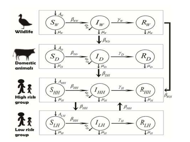 Figure 1. Emerging zoonotic pathogen transmission from wildlife, to domestic animals, to humans.
Emerging zoonotic pathogen transmission from wildlife, to domestic animals, to humans can be described as the model (2).
| {˙SW = AW−βWWIWSW−μWSW,˙IW=βWWIWSW−(μW+γW+αW)IW,˙RW=γWIW−μWRW,˙SD=AD−(βWDIW+βDDID)SD−μDSD,˙ID=(βWDIW+βDDID)SD−(γD+αD+μD)ID,˙RD=γDID−μDRD,˙SHH = AHH−[βWHIW+βDHID+βHH(IHH+ILH)]SHH−μHSHH,˙IHH=[βWHIW+βDHID+βHH(IHH+ILH)]SHH −(γH+αH+μH)IHH,˙RHH=γHIHH−μHRHH,˙SLH = ALH−βHH(IHH+ILH)SLH−μHSLH,˙ILH=βHH(IHH+ILH)SLH−(γH+αH+μH)ILH,˙RLH=γHILH−μHRLH. | (2) |
The basic model has been established to reflect the pathogen transmission from wildlife, to domestic animals, to humans as model (2). Next step, we take the isolation and slaughter strategies into consideration [22,23,8,31,2,25,18]. For wildlife, it is difficult to control them when a zoonosis is emerging. Lethal control, vaccination and fencing (physical barriers) are the primary approaches to limit the number of susceptibles in wildlife. In this paper, we take lethal control and fencing (physical barriers) as the strategies to compare the similar isolation and slaughter strategies in emerging zoonotic pathogen transmission.
| {˙SW = AW−βWWIWSW−(μW+δS)SW,˙IW=βWWIWSW−(μW+γW+αW+δI)IW,˙RW=γWIW−(μW+δR)RW,˙SD=AD−((1−θD)βWDIW+βDDID)SD−μDSD,˙ID=((1−θD)βWDIW+βDDID)SD−(γD+αD+μD)ID,˙RD=γDID−μDRD,˙SHH = AHH−[(1−θH)βWHIW+βDHID+βHH(IHH+ILH)]SHH −μHSHH,˙IHH=[(1−θH)βWHIW+βDHID+βHH(IHH+ILH)]SHH −(γH+αH+μH)IHH,˙RHH=γHIHH−μHRHH,˙SLH = ALH−βHH(IHH+ILH)SLH−μHSLH,˙ILH=βHH(IHH+ILH)SLH−(γH+αH+μH)ILH,˙RLH=γHILH−μHRLH. | (3) |
For domestic animals, we can manage them in their entire lives. It is no need to slaughter all of the susceptibles in domestic animals. We can quarantine all of the domestic animals, then isolate susceptibles and slaughter infectives.
| {˙SD=AD−(βWDIW+βDDID)SD−μDSD,˙ID=(βWDIW+βDDID)SD−(γD+αD+μD+ΔI)ID,˙RD=γDID−μDRD,˙SHH = AHH−[βWHIW+(1−ΘH)βDHID+βHH(IHH+ILH)]SHH −μHSHH,˙IHH=[βWHIW+(1−ΘH)βDHID+βHH(IHH+ILH)]SHH −(γH+αH+μH)IHH,˙RHH=γHIHH−μHRHH,˙SLH = ALH−βHH(IHH+ILH)SLH−μHSLH,˙ILH=βHH(IHH+ILH)SLH−(γH+αH+μH)ILH,˙RLH=γHILH−μHRLH. | (4) |
For humans, we could not 'slaughter' anyone no matter how serious they were infected with some kind of zoonoses. The quarantine and isolation may be the best method to limit the pathogen transmission except for vaccination. But the effect of quarantine and isolation strategies in humans are different from animals. For taking isolation strategies in animals, it is the susceptible humans, who are afraid of getting infected, to take the initiative and get away from susceptible animals. So the per capita incidence rate from animals to humans,
| {˙SHH = AHH−[βWHIW+βDHID+βHH(IHH+ILH)]SHH −μHSHH−φ(I)SHH+γH1OHH1,˙OHH1=φ(I)SHH−γH1OHH1−μHOHH1,˙IHH=[βWHIW+βDHID+βHH(IHH+ILH)]SHH −(γH+αH+μH+σ)IHH,˙OHH2=σIHH−γH2OHH2−μHOHH2,˙RHH=γHIHH+γH2OHH2−μHRHH,˙SLH = ALH−βHH(IHH+ILH)SLH−μHSLH −φ(I)SLH+γH1OLH1,˙OLH1=φ(I)SLH−γH1OLH1−μHOLH1,˙ILH=βHH(IHH+ILH)SLH−(γH+αH+μH+σ)ILH,˙OLH2=σILH−γH2OLH2−μHOLH2,˙RLH=γHILH+γH2OLH2−μHRLH. | (5) |
In conclusion, we can get the isolation and slaughter strategies controlling model by (3), (4) and (5) in wildlife, domestic animals and humans as the form:
| {˙SW = AW−βWWIWSW−(μW+εWδS)SW,˙IW=βWWIWSW−(μW+γW+αW+εWδI)IW,˙RW=γWIW−(μW+εWδR)RW,˙SD=AD−((1−εWθD)βWDIW+βDDID)SD−μDSD,˙ID=((1−εWθD)βWDIW+βDDID)SD −(γD+αD+μD+εDΔI)ID,˙RD=γDID−μDRD,˙SHH = AHH−[(1−εWθH)βWHIW+(1−εDΘH)βDHID+βHH(IHH +ILH)]SHH−μHSHH−εHφ(I)SHH+γH1OHH1,˙OHH1=εHφ(I)SHH−γH1OHH1−μHOHH1,˙IHH=[(1−εWθH)βWHIW+(1−εDΘH)βDHID +βHH(IHH+ILH)]SHH−(γH+αH+μH+εHσ)IHH,˙OHH2=εHσIHH−γH2OHH2−μHOHH2,˙RHH=γHIHH+γH2OHH2−μHRHH,˙SLH = ALH−βHH(IHH+ILH)SLH−μHSLH −εHφ(I)SLH+γH1OLH1,˙OLH1=εHφ(I)SLH−γH1OLH1−μHOLH1,˙ILH=βHH(IHH+ILH)SLH−(γH+αH+μH+εHσ)ILH,˙OLH2=εHσILH−γH2OLH2−μHOLH2,˙RLH=γHILH+γH2OLH2−μHRLH. | (6) |
with Strategy 1,
| {εW=0,ILH+IHH<IWCεW=1,ILH+IHH≥IWC | (7) |
Strategy 2,
| {εD=0,ILH+IHH<IDCεD=1,ILH+IHH≥IDC | (8) |
Strategy 3,
| {εH=0,ILH+IHH<IHCεH=1,ILH+IHH≥IHC | (9) |
The feasible set
Total number of wildlife is
It is difficult for us to take any strategies to control emerging zoonoses in first time. Only the infected of numbers of people would cause our attention to take some strategies to control the infectious disease. So it is assumed that if the number of infectives in human including high risk group and low risk group reached a threshold at
With
In (2), the wildlife class can be separated as
| {˙SW = AW−βWWIWSW−μWSW,˙IW=βWWIWSW−μWIW−γWIW−αWIW. | (10) |
We can get the basic reproductive number in wildlife
The disease-free equilibrium is
Theorem 2.1. If
Proof. The next generation matrix of the vector field corresponding to system (10) at
| JW(E0(W))=(−μW−βWWAWμW0βWWAWμW−μW−γW−αW) |
If
Similarly, the next generation matrix at
| JW(E∗(W))=(−βWWˆIW−μW−βWWˆSWβWWˆIWβWWˆSW−μW−γW−αW) |
The characteristic equation of
| fW(λ)=λ2+AWβWWμW+γW+αWλ+μW(μW+γW+αW)(AWβWWμW(μW+γW+αW)−1)=0 |
If
In (2), the wildlife and domestic animals classes can be separated as
| {˙SW = AW−βWWIWSW−μWSW,˙IW=βWWIWSW−μWIW−γWIW−αWIW,˙SD = AD−βWDIWSD−βDDIDSD−μDSD,˙ID=βWDIWSD+βDDIDSD−γDID−αDID−μDID. | (11) |
We can get the basic reproductive number in domestic animals is
The disease-free equilibrium is
Theorem 2.2. If
Proof. There always exists
| JWD(E0(WD))=(JW(E0(W))0∗JD(E0(D))) |
with
| JD(E0(D))=(−μD−βDDADμD0βDDADμD−μD−γD−αD) |
If
In (11), the epidemic equilibrium
| AW−βWWˆIWˆSW−μWˆSW = 0 | (12) |
| βWWˆIWˆSW−μWˆIW−γWˆIW−αWˆIW = 0 | (13) |
| AD−βWDˆIWˆSD−βDDˆIDˆSD−μDˆSD = 0 | (14) |
| βWDˆIWˆSD+βDDˆIDˆSD−μDˆID−γDˆID−αDˆID = 0 | (15) |
From (12), (13), (14), (15), we can get
| ˆSW=μW+γW+αWβWW |
| ˆIW=μWβWW(AWβWWμW(μW+γW+αW)−1) |
| ˆID = βWDˆIWˆSDμD+γD+αD−βDDˆSD=βWDˆSDμD+γD+αD−βDDˆSD×μWβWW(AWβWWμW(μW+γW+αW)−1) |
and
| ˆSD=12μDβDD[ADβDD+(μD+γD+αD)(μD+βWDˆIW)]−12μDβDD[A2Dβ2DD+2ADβDD(μD+γD+αD)(βWDˆIW−μD)+(μD+γD+αD)2(μD+βWDˆIW)2]12 |
So if
In fact, for
| g1(ˆSD)=μDβDDˆSD2−[ADβDD+(μD+γD+αD)(μD+βWDˆIW)]ˆSD+AD(μD+γD+αD)=0 |
If
So we choose
| ˆSD=12μDβDD[ADβDD+(μD+γD+αD)(μD+βWDˆIW)]−12μDβDD[A2Dβ2DD+2ADβDD(μD+γD+αD)(βWDˆIW−μD)+(μD+γD+αD)2(μD+βWDˆIW)2]12 |
to guarantee
The next generation matrix at
| JWD(E∗(WD))=(JW(E∗(W))0∗JD(E∗(D))) |
with
| JD(E∗(D))=(−βWDˆIW−βDDˆID−μD−βDDˆSDβWDˆIW+βDDˆIDβDDˆSD−μD−γD−αD) |
The characteristic equation of
If
In conclusion, if
The human class in (2) can be separated as the form:
| {˙SHH = AHH−βWHIWSHH−βDHIDSHH−βHH(IHH+ILH)SHH −μHSHH,˙IHH=βWHIWSHH+βDHIDSHH+βHH(IHH+ILH)SHH−γHIHH −αHIHH−μHIHH,˙SLH = ALH−βHH(IHH+ILH)SLH−μHSLH,˙ILH=βHH(IHH+ILH)SLH−γHILH−αHILH−μHILH. | (16) |
There always exists disease-free equilibrium
The next generation matrix at
| JWDH(E0(WDH))=(JW(E0(W))00∗JD(E0(D))0∗∗JH(E0(H))) |
with
| JH(E0(H))=(−μH−βHHAHHμH0−βHHAHHμH0βHHAHHμH−μH−γH−αH0βHHAHHμH0−βHHALHμH−μH−βHHALHμH0βHHALHμH0βHHALHμH−μH−γH−αH) |
The characteristic equation of
If there is
At the same time, the spectral radius of
Theorem 2.3. If
Proof. The next generation matrix at
| JWDH(E0(WDH))=(JW(E0(W))00∗JD(E0(D))0∗∗JH(E0(H))). |
If
Next we prove the existence of epidemic equilibrium
In (16), the epidemic equilibrium
| AHH−βWHˆIWˆSHH−βDHˆIDˆSHH−βHH(ˆIHH+ˆILH)ˆSHH−μHˆSHH = 0 | (17) |
| βWHˆIWˆSHH+βDHˆIDˆSHH+βHH(ˆIHH+ˆILH)ˆSHH−γHˆIHH−αHˆIHH−μHˆIHH = 0 | (18) |
| ALH−βHH(ˆIHH+ˆILH)ˆSLH−μHˆSLH = 0 | (19) |
| βHH(ˆIHH+ˆILH)ˆSLH−γHˆILH−αHˆILH−μHˆILH = 0 | (20) |
From (17) + (19), (18) + (20), we get
| AHH+ALH−βWHˆIWˆSHH−βDHˆIDˆSHH−βHH(ˆIHH+ˆILH)(ˆSHH+ˆSLH)−μH(ˆSHH+ˆSLH) = 0 | (21) |
| βWHˆIWˆSHH+βDHˆIDˆSHH+βHH(ˆIHH+ˆILH)(ˆSHH+ˆSLH)−(γH+αH+μH)(ˆIHH + ˆILH) = 0 | (22) |
It is assumed that
Then we have
| AHH+ALH−ηSβWHˆIWˆSH−ηSβDHˆIDˆSH−βHHˆIHˆSH−μHˆSH = 0 | (23) |
| ηSβWHˆIWˆSH+ηSβDHˆIDˆSH+βHHˆIHˆSH−(γH+αH+μH)ˆIH = 0 | (24) |
From (23), (24), we can get
| ˆIH = ηSβWHˆIWˆSH+ηSβDHˆIDˆSHγH+αH+μH−βHHˆSH |
and
| ˆSH=12μHβHH[(AHH+ALH)βHH+(γH+αH+μH)(μH+ηSβWHˆIW+ηSβDHˆID)]−12μHβHH[(AHH+ALH)2β2HH+2(AHH+ALH)βHH(γH+αH+μH)(ηSβWHˆIW+ηSβDHˆID−μH)+(γH+αH+μH)2(μH+ηSβWHˆIW+ηSβDHˆID)2]12 |
Similarly to the calculation of Theorem 2.2, we have
| g2(ˆSH)=μHβHHˆSH2+(AHH+ALH)(μH+γH+αH)−[(AHH+ALH)βHH+(μH+γH+αH)(μH+ηSβWHˆIW+ηSβDHˆID)]ˆSH=0 |
So if
| JWDH(E∗(WDH))=(JW(E∗(W))00∗JD(E∗(D))0∗∗JH(E∗(H))) |
with
| JH(E∗(H))=(J11−βHHˆSHH0−βHHˆSHHJ21J220βHHˆSHH0−βHHˆSLHJ33−βHHˆSLH0βHHˆSLHβHH(ˆIHH+ˆILH)J44) |
| J11=−βWHˆIW−βDHˆID−βHH(ˆILH+ˆILH)−μH |
| J21=βWHˆIW+βDHˆID+βHH(ˆILH+ˆILH) |
| J22=βHHˆSHH−γH−αH−μH |
| J33=−βHH(ˆIHH+ˆILH)−μH |
| J44=βHHˆSLH−γH−αH−μH |
The characteristic equation of
| fH2(λ)=λ4 + a1λ3+a2λ2 + a3λ + a4=0 |
with
| a1=AHHˆSHH+ALHˆSLH−βHH(ˆSHH+ˆSLH)+2(γH+αH+μH), |
| a2=(AHHˆSHH+ALHˆSLH)(γH+αH+μH)−μHβHH(ˆSHH+ˆSLH)−β2HHˆSHHˆSLH+(AHHˆSHH+βWHˆIWˆIHHˆSHH+βDHˆIDˆIHHˆSHH+βHHˆILHˆIHHˆSHH)(ALHˆSLH+βHHˆIHHˆILHˆSLH), |
| a3=ALHˆSLH(AHHˆSHH+γH+αH+μH)(γH+αH+μH)−μHβHHˆSLH(AHHˆSHH+γH+αH+μH)−βHHˆSHHALHˆSLH(γH+αH+μH)+AHHˆSHH(ALHˆSLH+γH+αH+μH)(γH+αH+μH)−μHβHHˆSHH(ALHˆSLH+γH+αH+μH)−βHHˆSLHAHHˆSHH(γH+αH+μH), |
| a4=AHHˆSHHALHˆSLH(γH+αH+μH)2−μHβHH(ˆSHHALHˆSLH+ˆSLHAHHˆSHH)(γH+αH+μH) |
It is assumed that
In conclusion, if
From Theorem 2.1, Theorem 2.2 and Theorem 2.3, it is more difficult to satisfy the conditions to control emerging zoonoses with the number of susceptible species increasing. But if there was an epidemic in wildlife with
Next we take Strategy 1, Strategy 2 and Strategy 3 into consideration in order to compare the effects of different isolation and slaughter strategies in wildlife, domestic animals and humans on emerging zoonoses.
Strategy 1.
It is assumed that
| {˙SW = AW−βWWIWSW−μWSW−δSW,˙IW=βWWIWSW−μWIW−γWIW−αWIW−δIW,˙RW=γWIW−μWRW−δRW,˙SD = AD−(1−θD)βWDIWSD−βDDIDSD−μDSD,˙ID=(1−θD)βWDIWSD+βDDIDSD−γDID−αDID−μDID,˙RD=γDID−μDRD,˙SHH = AHH−(1−θH)βWHIWSHH−βDHIDSHH−βHH(IHH +ILH)SHH−μHSHH,˙IHH=(1−θH)βWHIWSHH+βDHIDSHH+βHH(IHH+ILH)SHH −γHIHH−αHIHH−μHIHH,˙RHH=γHIHH−μHRHH,˙SLH = ALH−βHH(IHH+ILH)SLH−μHSLH,˙ILH=βHH(IHH+ILH)SLH−γHILH−αHILH−μHILH,˙RLH=γHILH−μHRLH. | (25) |
In (25), we get the control reproductive number in wildlife is
For the epidemic equilibrium of
Theorem 2.4. If
Strategy 2.
In (4), we get the control reproductive number in wildlife is
For the epidemic equilibrium of
In fact,
| g3(ˆS2D)=μDβDD(ˆS2D)2−[ADβDD+(μD+γD+αD+ΔI)(μD+βWDˆIW)]ˆS2D+AD(μD+γD+αD+ΔI)=0 |
So we have
| g3(ˆSD)=μDβDDˆSD2−[ADβDD+(μD+γD+αD+ΔI)(μD+βWDˆIW)]ˆSD+AD(μD+γD+αD+ΔI) |
If
| g1(ˆSD)=μDβDDˆSD2−[ADβDD+(μD+γD+αD)(μD+βWDˆIW)]ˆSD+AD(μD+γD+αD)=0 |
and
| AD−βWDˆIWˆSD−βDDˆIDˆSD−μDˆSD = 0, |
we get
| g3(ˆSD)=[ADβDD+(μD+γD+αD)(μD+βWDˆIW)]ˆSD−AD(μD+γD+αD)−[ADβDD+(μD+γD+αD+ΔI)(μD+βWDˆIW)]ˆSD+AD(μD+γD+αD+ΔI)=−ΔI(μD+βWDˆIW)ˆSD+ΔIAD=ΔIβDDˆIDˆSD>0. |
Then we get
Theorem 2.5. If
Strategy 3.
If we took quarantine and isolation strategies in humans only, the impact of wildlife and domestic animals in human epidemic would be never changed comparing to no strategy. So we select the human epidemic model (26) from (5) for further analysis. At the same time, we choose
| {˙SHH = AHH−βWHIWSHH−βDHIDSHH−βHH(IHH+ILH)SHH μHSHH−ρ(IHH+ ILH)SHH+γH1OHH1,˙OHH1=ρ(IHH+ ILH)SHH−γH1OHH1−μHOHH1,˙IHH=βWHIWSHH+βDHIDSHH+βHH(IHH+ILH)SHH −γHIHH−αHIHH−μHIHH−σIHH,˙OHH2=σIHH−γH2OHH2−μHOHH2,˙SLH = ALH−βHH(IHH+ILH)SLH−μHSLH−ρ(IHH+ ILH)SLH +γH1OLH1,˙OLH1=ρ(IHH+ ILH)SLH−γH1OLH1−μHOLH1,˙ILH=βHH(IHH+ILH)SLH−γHILH−αHILH−μHILH−σILH,˙OLH2=σILH−γH2OLH2−μHOLH2. | (26) |
We get the control reproductive number in humans is:
| R3(H)=(AHH+ALH)βHHμH(μH+γH+αH+σ) |
Theorem 2.6. If
| Strategies | no strategy | Strategy 1 | Strategy 2 | Strategy 3 |
| Reproductive number in wildlife | | |||
| Reproductive number in domestic animals | | | ||
| Reproductive number in humans | | | ||
 DownLoad: CSV
In this section we take avian influenza epidemic in China as an example to analyze the effects of different strategies on emerging zoonoses. Avian influenza is a kind of zoonoses, which have been prevalent in humans since 150 years ago. Avian influenza virus originated from aquatic birds, and it infected domestic birds by sharing watersheds. Humans can be infected by avian influenza virus via infected domestic birds[11,30,6,9]. But for birds, we cannot get the exact parameters to reflect the virus transmission clearly. So we take some similar data to estimate the process of avian influenza virus transmission approximately (TABLE 2).
| Parameter | Definitions | Values | Sources |
| birth or immigration rate of wild aquatic birds | 0.137 birds/day | Est. | |
| | natural mortality rate of wild aquatic birds | 0.000137/day | [33] |
| | recovery rate of wild aquatic birds | 0.25/day | Est. |
| | disease-induced mortality rate of wild aquatic birds | 0.0025/day | Est. |
| | birth or immigration rate of domestic birds | 48.72 birds/day | [33] |
| | natural mortality rate of domestic birds | 0.0058/day | [33] |
| | recovery rate of domestic birds | 0.25/day | [26] |
| | disease-induced mortality rate of domestic birds | 0.0025/day | Est. |
| | birth or immigration rate of humans | 0.07people/day | [23] |
| | natural mortality rate of humans | 0.000035/day | [23] |
| | recovery rate of humans | 0.33/day | [26, 31] |
| | remove rate from isolation compartment to susceptible compartment. | 0.5/day | Est. |
| | remove rate from isolation compartment to recovery individual compartment. | 0.5/day | Est. |
| | disease-induced mortality rate of humans | 0.0033/day | Est. |
| | basic reproductive number of wild aquatic birds | 2 | Est. |
| | basic reproductive number of domestic birds | 2 | Est. |
| | basic reproductive number of humans | 1.2 | [26] |
| | per capita incidence rate from wild aquatic birds to domestic birds | Est. | |
| | per capita incidence rate from wild aquatic birds to humans | Est. | |
| | per capita incidence rate from domestic birds to humans | Est. |
DownLoad: CSVThe number of domestic birds is 4.2 times more than the number of humans in China [7], so we assume that the number of domestic birds is 8400 and the number of humans is 2000 to simplify the calculation. And it is assumed that there are about 1000 wild aquatic birds for no exact data found. And it is assumed that
The avian influenza virus transmission has been shown in model (2), which included wildlife, domestic animals, high risk group and low risk group [10,21,13]. For high risk group and low risk group in humans, there may be shown in different proportion in different areas. Less people are needed to take care of live animals in modern farming than tradition. Few people have opportunities to contact with live animals in some areas, which are the potential hosts of some pathogens in emerging zoonoses. But in some other areas, stock raising is the main economy origin of the residents. More people have to look after live animals to help support the family. The proportion of high risk group and low risk group is higher in these areas than others. Here we choose different proportions of high risk group and low risk group, such as 1:9, 1:3, 1:1, 3:1 and 9:1, to reflect emerging avian influenza prevalence in different areas (FIGURE 2).
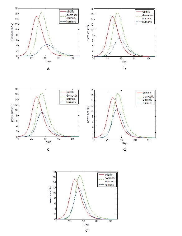 Figure 2. Avian influenza prevalence in wildlife, domestic animals and humans with high risk group: low risk group=1:9 in a, 1:3 in b, 1:1 in c, 3:1 in d 9:1 in e.
From a to e in FIGURE 2, we get that more and more high proportion of humans are infected in the first 90 days. More people would be infected with higher proportion of them having the opportunity to contact with susceptible animals. From FIGURE 3, we get that the incidence rate on epidemic equilibrium is increasing with higher proportion of high risk group in humans. Although the proportion of high risk group in humans would never change the basic reproductive number, it could impact the final prevalence in humans.
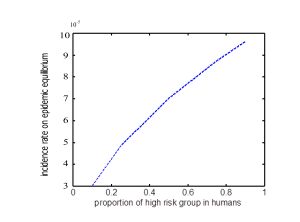 Figure 3. Incidence rate on epidemic equilibrium change in different proportion of high risk group in humans.
The effects of parameters
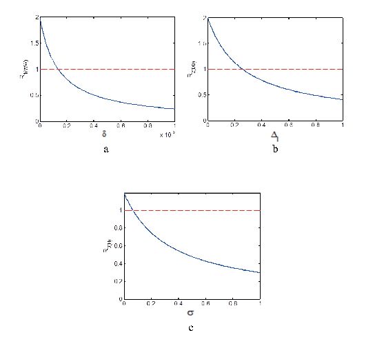 Figure 4. The effect of
 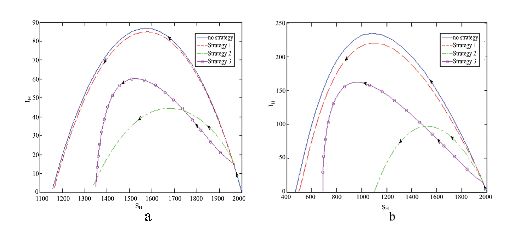 Figure 5. Phase portrait of
 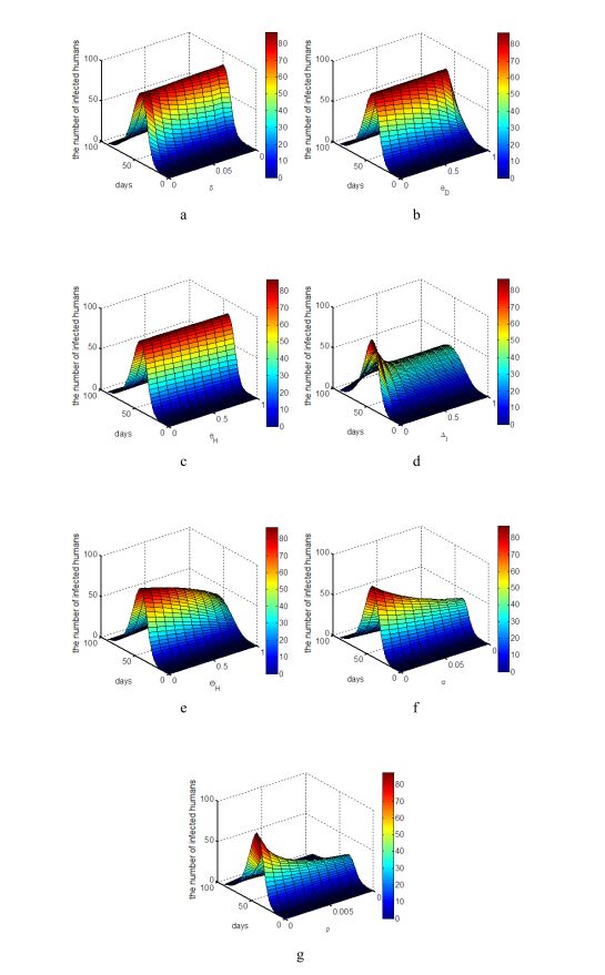 Figure 6. The effects of
 From Ebola, Hendra, Marburg, SARS to H1N1, H7N9, more and more zoonotic pathogens come into humans. Tens of thousands of people have dead of these zoonoses in the last hundreds of years. Some public health policies have to be established to answer emerging or remerging zoonoses. For different species participating in an emerging zoonosis, different strategies should been taken for controlling. In this paper, we established model (3), model (4) and model (5) to reflect the effects of Strategy 1, Strategy 2 and Strategy3 about isolation and slaughter in emerging zoonoses respectively. Strategy 1 is the controlling measure for wildlife. Strategy 2 is the controlling measure for domestic animals. And Strategy 3 is the controlling measure for humans.
All of the three strategies would change the basic reproductive number to their own control reproductive number. The involvement of Strategy 1, Strategy 2 and Strategy 3 would change the conditions, which determine the zoonoses prevalence or not. At the same time, we conclude that the extinction of zoonoses must satisfy the conditions ensuring all of basic (control) reproductive numbers in different species are less than 1, whether it is taken controlling strategy or not. But if and only if basic (control) reproductive numbers in wildlife is more than 1, the zoonoses might be prevalent in all of the susceptible species.
The stability analysis on models in section 2 reflects the effects of three strategies on control reproductive numbers and equilibriums. In section 3, some numerical simulations show the effects of the three strategies on avian influenza epidemic in different areas in China at beginning. In this paper, we take isolation and slaughter strategies into consideration to study their effects on emerging zoonoses. But the other effective strategies like vaccination are neglected, which could be proposed in a forthcoming paper.
This work was supported by the National Natural Science Foundation of China (11371048).
| [1] |
J. T. Bonner, M. E. Hoffman, Evidence for a substance responsible for the spacing pattern of aggregation and fruiting in the cellular slime molds, J. Embryol. Exp. Morphol., 11 (1963), 571–589. https://doi.org/10.1242/dev.11.3.571 doi: 10.1242/dev.11.3.571

|
| [2] |
C. S. Patlak, Random walk with persistence and external bias, Bull. Math. Biophys, 15 (1953), 311–338. https://doi.org/10.1007/BF02476407 doi: 10.1007/BF02476407
|
| [3] |
E. F. Keller, L. A. Segel, Initiation of slime mold aggregation viewed as an instability, J. Theor. Biol., 26 (1970), 399–415. https://doi.org/10.1016/0022-5193(70)90092-5 doi: 10.1016/0022-5193(70)90092-5
|
| [4] |
E. F. Keller, L. A. Segel, Model for chemotaxis, J. Theor. Biol., 30 (1971), 225–234. https://doi.org/10.1016/0022-5193(71)90050-6 doi: 10.1016/0022-5193(71)90050-6
|
| [5] |
E. F. Keller, L. A. Segel, Traveling bands of chemotactic bacteria: a theoretical analysis, J. Theor. Biol., 30 (1971), 235–248. https://doi.org/10.1016/0022-5193(71)90051-8 doi: 10.1016/0022-5193(71)90051-8
|
| [6] |
L. A. Segel, B. Stoeckly, Instability of a layer of chemostatic cells, attractant and degrading enzymes, J. Theor. Biol., 37 (1972), 561–585. https://doi.org/10.1016/0022-5193(72)90091-4 doi: 10.1016/0022-5193(72)90091-4
|
| [7] |
S. Childress, J. K. Percus, Nonlinear aspects of chemotaxis, Math. Biosci., 56 (1981), 217–237. https://doi.org/10.1016/0025-5564(81)90055-9 doi: 10.1016/0025-5564(81)90055-9
|
| [8] |
X. F. Chen, J. H. Hao, X. F. Wang, Y. P. Wu, Y. J. Zhang, Stability of spiky solution of Keller-Segel's minimal chemotaxis model, J. Differ. Equations, 257 (2014), 3102–3134. https://doi.org/10.1016/j.jde.2014.06.008 doi: 10.1016/j.jde.2014.06.008
|
| [9] |
T. Hillen, K. J. Painter, A user's guide to PDE models for chemotaxis, J. Math. Biol., 58 (2009), 183–217. https://doi.org/10.1007/s00285-008-0201-3 doi: 10.1007/s00285-008-0201-3
|
| [10] |
T. Hashira, S. Ishida, T. Yokota, Finite time blow-up for quasilinear degenerate Keller-Segel systems of parabolic-parabolic type, J. Differ. Equations, 264 (2018), 6459–6485. https://doi.org/10.1016/j.jde.2018.01.038 doi: 10.1016/j.jde.2018.01.038
|
| [11] |
L. Wang, Y. Li, C. Mu, Boundedness in a parabolic-parabolic quasilinear chemotaxis system with logistic source, Discrete Contin. Dyn. Syst., 34 (2014), 789–802. http://dx.doi.org/10.3934/dcds.2014.34.789 doi: 10.3934/dcds.2014.34.789
|
| [12] |
J. I. Tello, M. Winkler, A chemotaxis system with logistic source, Commun. Partial Differ. Equations, 32 (2007), 849–877. https://doi.org/10.1080/03605300701319003 doi: 10.1080/03605300701319003
|
| [13] | D. Horstmann, From 1970 until present: The Keller-Segel model in chemotaxis and its consequences Ⅰ, Jahresber. Dtsch. Math. Ver, 105 (2003), 103–165. |
| [14] | D. Horstmann, From 1970 until present: The Keller-Segel model in chemotaxis and its consequences Ⅰ, Jahresber. Dtsch. Math. Ver, 106 (2004), 51–69. |
| [15] |
G. Arumugam, J. Tyagi, Keller-Segel chemotaxis models: a review, Acta Appl. Math., 171 (2021), 1–82. https://doi.org/10.1007/s10440-020-00374-2 doi: 10.1007/s10440-020-00374-2
|
| [16] |
A. Chertock, A. Kurganov, A second-order positivity preserving central-upwind scheme for chemo-taxis and haptotaxis models, Numer. Math., 111 (2008), 169–205. https://doi.org/10.1007/s00211-008-0188-0 doi: 10.1007/s00211-008-0188-0
|
| [17] |
A. Chertock, Y. Epshteyn, H. Hu, A. Kurganov, High-order positivity-preserving hybrid finite-volume-finite-difference methods for chemotaxis systems, Adv. Comput. Math., 44 (2018), 327–350. https://doi.org/10.1007/s10444-017-9545-9 doi: 10.1007/s10444-017-9545-9
|
| [18] |
A. Adler, Chemotaxis in bacteria, Ann. Rev. Biochem, 44 (1975), 341–356. https://doi.org/10.1146/annurev.bi.44.070175.002013 doi: 10.1146/annurev.bi.44.070175.002013
|
| [19] |
E. O. Budrene, H. C. Berg, Complex patterns formed by motile cells of escherichia coli, Nature, 349 (1991), 630–633, https://doi.org/10.1038/349630a0 doi: 10.1038/349630a0
|
| [20] |
E. O. Budrene, H. C. Berg, Dynamics of formation of symmetrical patterns by chemotactic bacteria, Nature, 376 (1995), 49–53. https://doi.org/10.1038/376049a0 doi: 10.1038/376049a0
|
| [21] |
M. H. Cohen, A. Robertson, Wave propagation in the early stages of aggregation of cellular slime molds, J. Theor. Biol., 31 (1971), 101–118. https://doi.org/10.1016/0022-5193(71)90124-X doi: 10.1016/0022-5193(71)90124-X
|
| [22] |
V. Nanjundiah, Chemotaxis, signal relaying and aggregation morphology, J. Theor. Biol., 42 (1973), 63–105. https://doi.org/10.1016/0022-5193(73)90149-5 doi: 10.1016/0022-5193(73)90149-5
|
| [23] |
X. Wang, Q. Xu, Spiky and transition layer steady states of chemotaxis systems via global bifurcation and Helly's compactness theorem, J. Math. Biol., 66 (2013), 1241–1266. https://doi.org/10.1007/s00285-012-0533-x doi: 10.1007/s00285-012-0533-x
|
| [24] |
E. Feireisl, P. Laurençot, H. Petzeltová, On convergence to equilibria for the Keller-Segel chemotaxis model, J. Differ. Equations, 236 (2007), 551–569. https://doi.org/10.1016/j.jde.2007.02.002 doi: 10.1016/j.jde.2007.02.002
|
| [25] |
T. Hillen, A. Potapov, The one-dimensional chemotaxis model global existence and asymptotic profile, Math. Method Appl. Sci., 27 (2004), 1783–1801. https://doi.org/10.1002/mma.569 doi: 10.1002/mma.569
|
| [26] | K. Osaki, A. Yagi, Finite dimensional attractor for one-dimensional Keller-Segel equations, Funkcialaj Ekvacioj, 44 (2001), 441–469. |
| [27] |
X. F. Xiao, X. L. Feng, Y. N. He, Numerical simulations for the chemotaxis models on surfaces via a novel characteristic finite element method, Comput. Math. Appl., 78 (2019), 20–34. https://doi.org/10.1016/j.camwa.2019.02.004 doi: 10.1016/j.camwa.2019.02.004
|
| [28] |
X. Li, C. W. Shu, Y. Yang, Local discontinuous Galerkin method for the Keller-Segel chemotaxis model, J. Sci. Comput., 73 (2017), 943–967. https://doi.org/10.1007/s10915-016-0354-y doi: 10.1007/s10915-016-0354-y
|
| [29] |
L. Guo, X. Li, Y. Yang, Energy dissipative local discontinuous Galerkin methods for Keller-Segel chemotaxis model, J. Sci. Comput., 78 (2019), 1387–1404. https://doi.org/10.1007/s10915-018-0813-8 doi: 10.1007/s10915-018-0813-8
|
| [30] |
Y. Epshteyn, A. Izmirlioglu, Fully discrete analysis of a discontinuous finite element method for the Keller-Segel chemotaxis model, J. Sci. Comput., 40 (2009), 211–256. https://doi.org/10.1007/s10915-009-9281-5 doi: 10.1007/s10915-009-9281-5
|
| [31] |
Y. Epshteyn, A. Kurganov, New interior penalty discontinuous galerkin methods for the Keller-Segel chemotaxis model, SIAM J. Numer. Anal., 47 (2008), 386–408. https://doi.org/10.1137/07070423X doi: 10.1137/07070423X
|
| [32] |
M. Sulman, T. Nguyen, A positivity preserving moving mesh finite element method for the Keller-Segel chemotaxis model, J. Sci. Comput., 80 (2019), 649–666. https://doi.org/10.1007/s10915-019-00951-0 doi: 10.1007/s10915-019-00951-0
|
| [33] |
C. Qiu, Q. Liu, J. Yan, Third order positivity-preserving direct discontinuous Galerkin method with interface correction for chemotaxis Keller-Segel equations, J. Comput. Phys., 433 (2021), 110191. https://doi.org/10.1016/j.jcp.2021.110191 doi: 10.1016/j.jcp.2021.110191
|
| [34] |
F. Filbet, A finite volume scheme for the Patlak-Keller-Segel chemotaxis model, Numerisch Math., 104 (2006), 457–488. https://doi.org/10.1007/s00211-006-0024-3 doi: 10.1007/s00211-006-0024-3
|
| [35] |
A. Kurganov, E. Tadmor, New high-resolution central schemes for nonlinear conservation laws and convection-diffusion equations, J. Comput. Phys., 160 (2000), 241–282. https://doi.org/10.1006/jcph.2000.6459 doi: 10.1006/jcph.2000.6459
|
| [36] |
Y. Epshteyn, Upwind-difference potentials method for Patlak-Keller-Segel chemotaxis model, J. Sci. Comput., 53 (2012), 689–713. https://doi.org/10.1007/s10915-012-9599-2 doi: 10.1007/s10915-012-9599-2
|
| [37] |
R. Tyson, L. G. Stern, R. J. LeVeque, Fractional step methods applied to a chemotaxis model, J. Math. Biol., 41 (2000), 455–475. https://doi.org/10.1007/s002850000038 doi: 10.1007/s002850000038
|
| [38] |
D. Manoussaki, A mechanochemical model of angiogenesis and vasculogenesis, Math. Model. Numer. Anal., 37 (2003), 581–599. https://doi.org/10.1007/10.1051/m2an:2003046 doi: 10.1007/10.1051/m2an:2003046
|
| [39] |
N. Saito, T. Suzuki, Notes on finite difference schemes to a parabolic-elliptic system modelling chemotaxis, Appl. Math. Comput., 171 (2005), 72–90. https://doi.org/10.1016/j.amc.2005.01.037 doi: 10.1016/j.amc.2005.01.037
|
| [40] | N. Saito, Conservative numerical schemes for the Keller-Segel system and numerical results, RIMS Kôkyûroku Bessatsu, 15 (2009), 125–146. |
| [41] |
A. Acrivos, Heat transfer at high Pclet number from a small sphere freely rotating in a simple shear field, J. Fluid Mech., 46 (2006), 233–240. https://doi.org/10.1017/S0022112071000508 doi: 10.1017/S0022112071000508
|
| [42] |
D. Liu, H. L. Han, Y. L. Zheng, A high-order method for simulating convective planar Poiseuille flow over a heated rotating sphere, Int. J. Numer. Methods Heat Fluid Flow, 28 (2018), 1892–1929. https://doi.org/10.1108/HFF-12-2017-0525 doi: 10.1108/HFF-12-2017-0525
|
| [43] | C. Gear, Numerical initial value problems in ordinary differential equations, Prentice Hall, 1971. |
| [44] |
G. H. Gao, Z. Z. Sun, Compact difference schemes for heat equation with Neumann boundary conditions Ⅰ, Numer. Method Partial Differ. Equations, 29 (2013), 1459–1486. https://doi.org/10.1002/num.21760 doi: 10.1002/num.21760
|
| [45] |
X. D. Liu, S. Osher, Nonoscillatory high order accurate self-similar maximum principle satisfying shock capturing schemes Ⅰ, SIAM J. Numer. Anal., 33 (1996), 760–779. https://doi.org/10.1137/0733038 doi: 10.1137/0733038
|
| [46] |
X. Zhang, C. W. Shu, Maximum-principle-satisfying and positivity-preserving high-order schemes for conservation laws: survey and new developments, Proc. R. Soc. A, 467 (2011), 2752–2776. https://doi.org/10.1098/rspa.2011.0153 doi: 10.1098/rspa.2011.0153
|
| [47] |
S. A. Orszag, M. Israelt, Numerical Simulation of Viscous Incompressible Flows, Ann. Rev. Fluid Mech., 6 (1974), 281–318. https://doi.org/10.1146/annurev.fl.06.010174.001433 doi: 10.1146/annurev.fl.06.010174.001433
|
| [48] |
S. K. Lele, Compact finite difference schemes with spectral-like resolution, J. Comput. Phys., 103 (1992), 16–42. https://doi.org/10.1016/0021-9991(92)90324-R doi: 10.1016/0021-9991(92)90324-R
|
| [49] |
T. Wang, T. G. Liu, A consistent fourth-order compact scheme for solving convection-diffusion equation, Math. Numerica Sinica, 38 (2016), 391–404. https://doi.org/10.12286/jssx.2016.4.391 doi: 10.12286/jssx.2016.4.391
|
| [50] | L. H. Thomas, Elliptic problems in linear difference equations over a network, Watson Sci. Comput. Lab. Columbia Univ., 1 (1949). |
| 1. | Yin Li, Ian Robertson, The epidemiology of swine influenza, 2021, 1, 2731-0442, 10.1186/s44149-021-00024-6 | |
| 2. | Fangyuan Chen, Zoonotic modeling for emerging avian influenza with antigenic variation and (M+1)–patch spatial human movements, 2023, 170, 09600779, 113433, 10.1016/j.chaos.2023.113433 |


Figures(11) / Tables(7)

Lin Zhang, Yongbin Ge, Zhi Wang. Positivity-preserving high-order compact difference method for the Keller-Segel chemotaxis model[J]. Mathematical Biosciences and Engineering, 2022, 19(7): 6764-6794. doi: 10.3934/mbe.2022319

| Strategies | no strategy | Strategy 1 | Strategy 2 | Strategy 3 |
| Reproductive number in wildlife | | |||
| Reproductive number in domestic animals | | | ||
| Reproductive number in humans | | | ||
DownLoad: CSV| Parameter | Definitions | Values | Sources |
| birth or immigration rate of wild aquatic birds | 0.137 birds/day | Est. | |
| | natural mortality rate of wild aquatic birds | 0.000137/day | [33] |
| | recovery rate of wild aquatic birds | 0.25/day | Est. |
| | disease-induced mortality rate of wild aquatic birds | 0.0025/day | Est. |
| | birth or immigration rate of domestic birds | 48.72 birds/day | [33] |
| | natural mortality rate of domestic birds | 0.0058/day | [33] |
| | recovery rate of domestic birds | 0.25/day | [26] |
| | disease-induced mortality rate of domestic birds | 0.0025/day | Est. |
| | birth or immigration rate of humans | 0.07people/day | [23] |
| | natural mortality rate of humans | 0.000035/day | [23] |
| | recovery rate of humans | 0.33/day | [26, 31] |
| | remove rate from isolation compartment to susceptible compartment. | 0.5/day | Est. |
| | remove rate from isolation compartment to recovery individual compartment. | 0.5/day | Est. |
| | disease-induced mortality rate of humans | 0.0033/day | Est. |
| | basic reproductive number of wild aquatic birds | 2 | Est. |
| | basic reproductive number of domestic birds | 2 | Est. |
| | basic reproductive number of humans | 1.2 | [26] |
| | per capita incidence rate from wild aquatic birds to domestic birds | Est. | |
| | per capita incidence rate from wild aquatic birds to humans | Est. | |
| | per capita incidence rate from domestic birds to humans | Est. |
DownLoad: CSV| Strategies | no strategy | Strategy 1 | Strategy 2 | Strategy 3 |
| Reproductive number in wildlife | | |||
| Reproductive number in domestic animals | | | ||
| Reproductive number in humans | | | ||
| Parameter | Definitions | Values | Sources |
| birth or immigration rate of wild aquatic birds | 0.137 birds/day | Est. | |
| | natural mortality rate of wild aquatic birds | 0.000137/day | [33] |
| | recovery rate of wild aquatic birds | 0.25/day | Est. |
| | disease-induced mortality rate of wild aquatic birds | 0.0025/day | Est. |
| | birth or immigration rate of domestic birds | 48.72 birds/day | [33] |
| | natural mortality rate of domestic birds | 0.0058/day | [33] |
| | recovery rate of domestic birds | 0.25/day | [26] |
| | disease-induced mortality rate of domestic birds | 0.0025/day | Est. |
| | birth or immigration rate of humans | 0.07people/day | [23] |
| | natural mortality rate of humans | 0.000035/day | [23] |
| | recovery rate of humans | 0.33/day | [26, 31] |
| | remove rate from isolation compartment to susceptible compartment. | 0.5/day | Est. |
| | remove rate from isolation compartment to recovery individual compartment. | 0.5/day | Est. |
| | disease-induced mortality rate of humans | 0.0033/day | Est. |
| | basic reproductive number of wild aquatic birds | 2 | Est. |
| | basic reproductive number of domestic birds | 2 | Est. |
| | basic reproductive number of humans | 1.2 | [26] |
| | per capita incidence rate from wild aquatic birds to domestic birds | Est. | |
| | per capita incidence rate from wild aquatic birds to humans | Est. | |
| | per capita incidence rate from domestic birds to humans | Est. |
