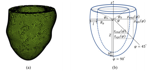
Estimating material properties of personalized human left ventricular (LV) modelling is a central problem in biomechanical studies. In this work we use deep learning (DL) method to evaluating the passive myocardial mechanical properties inversely. In the first part of the paper, we establish a standardized geometric model of the LV. The geometric model parameters are optimized based on 27 different healthy volunteers. In the second part, we use statistical methods and Latin hypercube sampling (LHS) to obtain the geometric parameters data. The LV myocardium is described using a structure-based orthotropic Holzapfel-Ogden constitutive law. The LV diastolic pressure-volume (PV) curves are calculated by numerical simulation. Tn the third part, we establish the multiple neural networks to pblackict PV curve parameters. Then, instead of using constrained optimization problems to solve constitutive parameters, DL was used to establish the nonlinear mapping relationship of geometric parameters, PV curve parameters and constitutive parameters. The results show that the deep learning method can greatly improve the computational efficiency of numerical simulation and increase the possibility of its application in rapid feedback of clinical data.
Citation: Li Cai, Jie Jiao, Pengfei Ma, Wenxian Xie, Yongheng Wang. Estimation of left ventricular parameters based on deep learning method[J]. Mathematical Biosciences and Engineering, 2022, 19(7): 6638-6658. doi: 10.3934/mbe.2022312
Estimating material properties of personalized human left ventricular (LV) modelling is a central problem in biomechanical studies. In this work we use deep learning (DL) method to evaluating the passive myocardial mechanical properties inversely. In the first part of the paper, we establish a standardized geometric model of the LV. The geometric model parameters are optimized based on 27 different healthy volunteers. In the second part, we use statistical methods and Latin hypercube sampling (LHS) to obtain the geometric parameters data. The LV myocardium is described using a structure-based orthotropic Holzapfel-Ogden constitutive law. The LV diastolic pressure-volume (PV) curves are calculated by numerical simulation. Tn the third part, we establish the multiple neural networks to pblackict PV curve parameters. Then, instead of using constrained optimization problems to solve constitutive parameters, DL was used to establish the nonlinear mapping relationship of geometric parameters, PV curve parameters and constitutive parameters. The results show that the deep learning method can greatly improve the computational efficiency of numerical simulation and increase the possibility of its application in rapid feedback of clinical data.

| [1] |
H. Gao, K. Mangion, D. Carrick, D. Husmeier, X. Y. Luo, C. Berry, Estimating prognosis in patients with acute myocardial infarction using personalized computational heart models, Sci. Rep., 7 (2017), 13527. https://doi.org/10.5465/AMBPP.2017.13527abstract doi: 10.5465/AMBPP.2017.13527abstract

|
| [2] |
K. Mangion, H. Gao, D. Husmeier, X. Y. Luo, C. Berry, Advances in computational modelling for personalised medicine after myocardial infarction, Heart (British Cardiac Society), 104 (2018), 550–557. https://doi.org/10.1136/heartjnl-2017-311449 doi: 10.1136/heartjnl-2017-311449
|
| [3] |
D. D. Streeter, W. T. Hanna, Engineering mechanics for successive states in canine left ventricular myocardium, Circ. Res., 33 (1973), 639–55. https://doi.org/10.1161/01.RES.33.6.639 doi: 10.1161/01.RES.33.6.639
|
| [4] |
S. F. Pravdin, V. I. Berdyshev, A. V. Panfilov, L. B. Katsnelson, V. S. Markhasin, Mathematical model of the anatomy and fibre orientation field of the left ventricle of the heart, Biomed. Eng. Online, 12 (2013), 54. https://doi.org/10.1186/1475-925X-12-54 doi: 10.1186/1475-925X-12-54
|
| [5] |
P. D. Achille, A. Harouni, S. Khamzin, O. Solovyova, J. J. Rice, Gaussian process regressions for inverse problems and parameter searches in models of ventricular mechanics, Front. Physiol., 9 (2018), 1002. https://doi.org/10.3389/fphys.2018.01002 doi: 10.3389/fphys.2018.01002
|
| [6] |
P. Gould, D. Ghista, L. Brombolich, I. Mirsky, In vivo stresses in the human left ventricular wall: Analysis accounting for the irregular 3-dimensional geometry and comparison with idealised geometry analyses, J. Biomech., 5 (1972), 521–539. https://doi.org/10.1016/0021-9290(72)90009-7 doi: 10.1016/0021-9290(72)90009-7
|
| [7] |
M. Sermesant, P. Moireau, O. Camara, J. S. Marie, R. Andriantsimiavona, R. Cimrman, et al., Cardiac function estimation from MRI using a heart model and data assimilation: advances and difficulties, Med. Image Anal., 10 (2006), 642–656. https://doi.org/10.1016/j.media.2006.04.002 doi: 10.1016/j.media.2006.04.002
|
| [8] |
C. S. Peskin, Flow patterns around heart valves: A numerical method, J. Comput. Phys., 10 (1972), 252–271. https://doi.org/10.1016/0021-9991(72)90065-4 doi: 10.1016/0021-9991(72)90065-4
|
| [9] |
L. Cai, H. Gao, X. Y. Luo, Y. F. Nie, Multi-scale modelling of the human left ventricle, Sci. Sin., 45 (2015), 024702. https://doi.org/10.1360/SSPMA2013-00100 doi: 10.1360/SSPMA2013-00100
|
| [10] |
B. E. Griffith, X. Y. Luo, Hybrid finite difference/finite element immersed boundary method, Int. J. Numer. Methods Biomed. Eng., 33 (2017), 101002. https://doi.org/10.1002/cnm.2888 doi: 10.1002/cnm.2888
|
| [11] |
H. Gao, H. M. Wang, C. Berry, X. Y. Luo, B. E. Griffith, Quasi-static imaged-based immersed boundary-finite element model of human left ventricle in diastole, John Wiley Sons. Ltd., 30 (2014), 1199–1222. https://doi.org/10.1002/cnm.2652 doi: 10.1002/cnm.2652
|
| [12] |
L. Cai, H. Gao, X. Y. Luo, Y. H. Wang, Y. Q. Li, A mathematical model for active contraction in healthy and failing myocytes and left ventricles, Plos One, 12 (2017), e0174834. https://doi.org/10.1371/journal.pone.0174834 doi: 10.1371/journal.pone.0174834
|
| [13] |
L. C. Yann, B. Yoshua, H. Geoffrey, Deep learning, Nature, 521 (2015), 436–44. https://doi.org/10.1038/nature14539 doi: 10.1038/nature14539
|
| [14] |
G. Litjens, T. Kooi, B. E. Bejnordi, A. Setio, C. I. Sánchez, A survey on deep learning in medical image analysis, Med. Image Anal., 42 (2017), 60–88. https://doi.org/10.1016/j.media.2017.07.005 doi: 10.1016/j.media.2017.07.005
|
| [15] |
D. Shen. G. Wu, H. I. Suk, A survey on deep learning in medical image analysis, Annu. Rev. Biomed. Eng., 19 (2017), 221–248. https://doi.org/10.1146/annurev-bioeng-071516-044442 doi: 10.1146/annurev-bioeng-071516-044442
|
| [16] | C. Case, J. Casper, G. Diamos, Deep Speech: Scaling up end-to-end speech recognition, Comput. Sci., 2014. |
| [17] |
J. Bonnemain, L. Pegolotti, L. Liaudet, S. Deparis, Implementation and calibration of a deep neural network to predict parameters of left ventricular systolic function based on pulmonary and systemic arterial pressure signals, Front. Physiol., 11 (2022), 1086. https://doi.org/10.3389/fphys.2020.01086 doi: 10.3389/fphys.2020.01086
|
| [18] |
J. Bonnemain, M. Zeller, L. Pegolotti, S. Deparis, L. Liaudet, Deep neural network to accurately predict left ventricular systolic function under mechanical assistance, Front. Cardiovasc. Med., 8 (2021), 752088. https://doi.org/10.3389/fcvm.2021.752088 doi: 10.3389/fcvm.2021.752088
|
| [19] |
L. Cai, L. Ren, Y. H. Wang, W. X. Xie, H. Gao, Surrogate models based on machine learning methods for parameter estimation of left ventricular myocardium, R. Soc. Open Sci., 8 (2021), 201121. https://doi.org/10.1098/rsos.201121 doi: 10.1098/rsos.201121
|
| [20] |
M. L. Liu, L. Liang, W. Sun, Estimation of in vivo constitutive parameters of the aortic wall: a machine learning approach, Comput. Methods Appl. Mech. Eng., 347 (2018), 201–217. https://doi.org/10.1016/j.cma.2018.12.030 doi: 10.1016/j.cma.2018.12.030
|
| [21] |
H. Gao, W. G. Li, L. Cai, C. Berry, X. Y. Luo, Parameter estimation in a Holzapfel-Ogden law for healthy myocardium, J. Eng. Math., 95 (2015), 231–248. https://doi.org/10.1007/s10665-014-9740-3 doi: 10.1007/s10665-014-9740-3
|
| [22] |
H. Gao, A. Aderhold, K. Mangion, Changes and classification in myocardial contractile function in the left ventricle following acute myocardial infarction, J. R. Soc. Interf., 14 (2017), 20170203. https://doi.org/10.1098/rsif.2017.0203 doi: 10.1098/rsif.2017.0203
|
| [23] |
S. F. Pravdin, H. Dierckx, L. B. Katsnelson, O. Solovyova, V. S. Markhasin, A. V. Panfilov, Electrical wave propagation in an anisotropic model of the left ventricle based on analytical description of cardiac architecture, Plos One, 9 (2014), e93617. https://doi.org/10.1371/journal.pone.0093617 doi: 10.1371/journal.pone.0093617
|
| [24] |
G. A. Holzapfel, R. W. Ogden, Constitutive modelling of passive myocardium: a structurally based framework for material characterization, Philos. Trans., 367 (2009), 3445–3475. https://doi.org/10.1098/rsta.2009.0091 doi: 10.1098/rsta.2009.0091
|
| [25] |
H. M. Wang, H. Gao, X. Y. Luo, C. Berry, B. E. Griffith, R. W. Ogden, et al., Structure-based finite strain modelling of the human left ventricle in diastole, Int. J. Numer. Methods Biomed. Eng., 29 (2013), 83–103. https://doi.org/10.37059/tjosal.2013.29.1.83 doi: 10.37059/tjosal.2013.29.1.83
|
| [26] |
L. Fan, J. Yao, C. Yang, D. Xu, D. Tang, Patient-specific echo-based left ventricle models for active contraction and relaxation using different zero-load diastole and systole geometries, Int. J. Comput. Methods, 16 (2017), 1842014. https://doi.org/10.1142/S0219876218420148 doi: 10.1142/S0219876218420148
|
| [27] |
G. Viatcheslav, A high-resolution computational model of the deforming human heart, Biomech. Model. Mechanobiol., 14 (2015), 829–849. https://doi.org/10.1007/s10237-014-0639-8 doi: 10.1007/s10237-014-0639-8
|
| [28] | Y. Xu, Simulation on the Mechanic Behaviour of Heart Based on Finite Element Methods, Ph.D thesis, Harbin Institute of Technology in Harbin, 2015. |
| [29] |
M. D. Mckay, R. J. Conover, J. Beckmanw, A comparison of three methods for selecting values of input variables in the analysis of output from a computer code, Technometrics, 21 (1979), 239–245. https://doi.org/10.2307/1268522 doi: 10.2307/1268522
|
| [30] |
K. Stefan, Single-beat estimation of end-diastolic pressure-volume relationship: a novel method with potential for noninvasive application, Am. J. Physiol., 291 (2006), H403–H412. https://doi.org/10.1152/ajpheart.01240.2005 doi: 10.1152/ajpheart.01240.2005
|
| [31] | G. Xavier, B. Antoine, B. Yoshua, Deep sparse rectifier neural networks, J. Mach. Learn. Res., 15 (2011), 315–323. |
| [32] |
G. A. Montague, M. T. Tham, M. J. Willis, A. J. Morris, Predictive control of distillation columns using dynamic neural networks, IFAC Proceed. Vol., 25 (1992), 243–248. https://doi.org/10.1016/S1474-6670(17)50999-4 doi: 10.1016/S1474-6670(17)50999-4
|
| [33] |
M. D. Mckay, R. J. Conover, J. Beckmanw, Adam: A method for stochastic optimization, CoRR, 2014. https://doi.org/10.48550/arXiv.1412.6980 doi: 10.48550/arXiv.1412.6980
|


Figures(13) / Tables(9)

Li Cai, Jie Jiao, Pengfei Ma, Wenxian Xie, Yongheng Wang. Estimation of left ventricular parameters based on deep learning method[J]. Mathematical Biosciences and Engineering, 2022, 19(7): 6638-6658. doi: 10.3934/mbe.2022312


 DownLoad: