The majority of stroke survivors suffer from physical and mental disabilities. This causes social and economic burdens, and it is regarded as a major source of morbidity and the second leading cause of death worldwide. This study aims to quantify the incidence of cerebrovascular stroke in the Taif region, identify risk factors for CVA, and raise awareness about modifiable risk factors.
Over 17 months period (February 2020 to June 2021), all first-stroke patients admitted to Alhada military hospital and King Faisal hospital in Taif region were included. Stroke patients from outside the Taif region were excluded from participating in the study. Age, gender, domicile, employment, history of hypertension, diabetes, cardiac diseases, smoking, previous history of stroke or transient ischemic episodes were all obtained from the patient's files. Also, a history of medications, particularly anticoagulants and contraceptive tablets if a female in childbearing age.
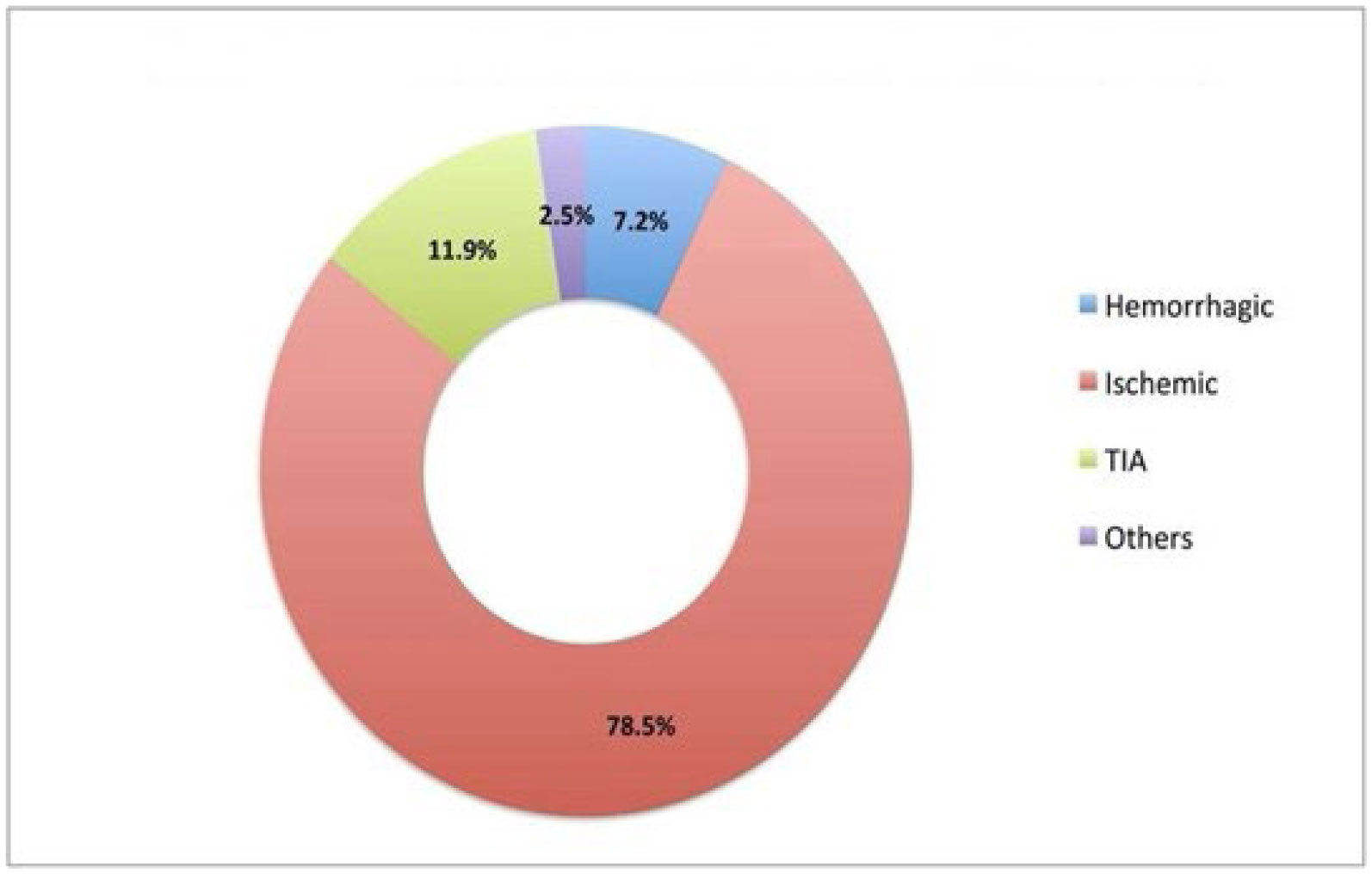
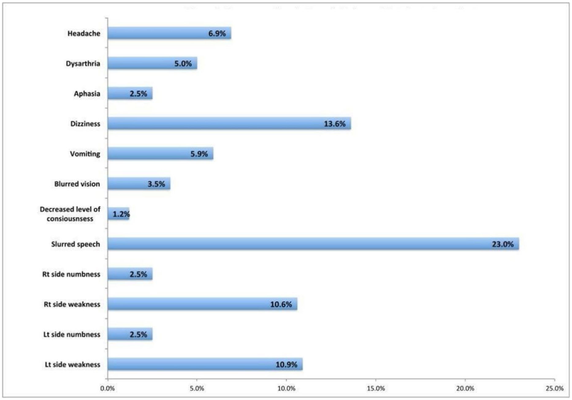
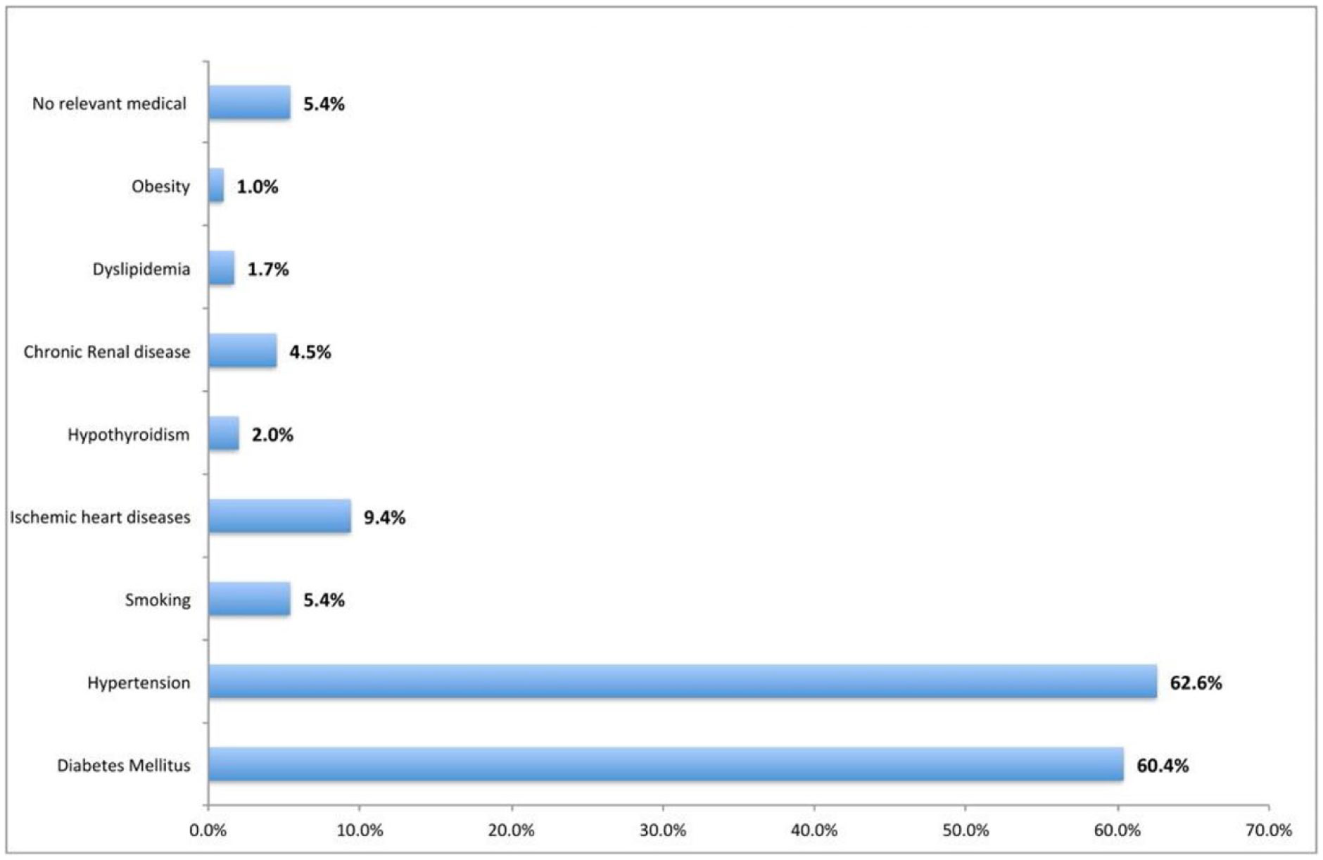
Overall, the study included 404 patients, 40.6% of whom were females and 59.4% of whom were males, with a mean age of 64.0 ± 14.9 years. The most common type of CVA was ischemic stroke (78.5%), followed by TIA (11.9%), and hemorrhagic stroke (7.2%). Slurred speech was the most commonly reported chief symptom among stroke survivors (23%), followed by dizziness (13.6%), left-sided weakness (10.9%), and right-sided weakness (10.9%). The incidence of stroke is increasing in patients who had chronic diseases like hypertension which is 62.6% survival had, and the second most common lead to stroke and decreased elasticity of vessels is diabetes mellitus 60.4% followed by ischemic heart disease 9.4% and smoking 5.4%.
Finally, using a prospective clinical study, the incidence of first time CVA in Taif was higher in males (about 59.4%) than in females (40.6%). That indicates a strong relation between Diabetes which represents 60.4%, Hypertension was 62.6% and age 18–55. We suggest running campaigns that target people with these risk factors to reduce the possibility of CVA occurrence.
Citation: Ola Shawky, Maha Alkhaldi, Deema Yousef, Adnan Alhindi, Teef Alosaimi, Amjad Jawhari, Aliah Aladwani. Incidence of first-time stroke in Taif, Saudi Arabia[J]. AIMS Medical Science, 2022, 9(2): 293-303. doi: 10.3934/medsci.2022012
The majority of stroke survivors suffer from physical and mental disabilities. This causes social and economic burdens, and it is regarded as a major source of morbidity and the second leading cause of death worldwide. This study aims to quantify the incidence of cerebrovascular stroke in the Taif region, identify risk factors for CVA, and raise awareness about modifiable risk factors.
Over 17 months period (February 2020 to June 2021), all first-stroke patients admitted to Alhada military hospital and King Faisal hospital in Taif region were included. Stroke patients from outside the Taif region were excluded from participating in the study. Age, gender, domicile, employment, history of hypertension, diabetes, cardiac diseases, smoking, previous history of stroke or transient ischemic episodes were all obtained from the patient's files. Also, a history of medications, particularly anticoagulants and contraceptive tablets if a female in childbearing age.
Overall, the study included 404 patients, 40.6% of whom were females and 59.4% of whom were males, with a mean age of 64.0 ± 14.9 years. The most common type of CVA was ischemic stroke (78.5%), followed by TIA (11.9%), and hemorrhagic stroke (7.2%). Slurred speech was the most commonly reported chief symptom among stroke survivors (23%), followed by dizziness (13.6%), left-sided weakness (10.9%), and right-sided weakness (10.9%). The incidence of stroke is increasing in patients who had chronic diseases like hypertension which is 62.6% survival had, and the second most common lead to stroke and decreased elasticity of vessels is diabetes mellitus 60.4% followed by ischemic heart disease 9.4% and smoking 5.4%.
Finally, using a prospective clinical study, the incidence of first time CVA in Taif was higher in males (about 59.4%) than in females (40.6%). That indicates a strong relation between Diabetes which represents 60.4%, Hypertension was 62.6% and age 18–55. We suggest running campaigns that target people with these risk factors to reduce the possibility of CVA occurrence.

| [1] |
Murray CJ, Vos T, Lozano R, et al. (2013) Disability-adjusted life years (DALYs) for 291 diseases and injuries in 21 regions, 1990–2010: a systematic analysis for the global burden of disease study 2010. Lancet 380: 2197-2223. https://doi.org/10.1016/S0140-6736(12)61689-4 
|
| [2] |
Ovbiagele B, Nguyen-Huynh MN (2011) Stroke epidemiology: advancing our understanding of disease mechanism and therapy. Neurotherapeutics 8: 319-329. https://doi.org/10.1007/s13311-011-0053-1
|
| [3] |
Thrift AG, Thayabaranathan T, Howard G, et al. (2017) Global stroke statistics. Int J Stroke 12: 13-32. https://doi.org/10.1177/1747493016676285
|
| [4] |
Benjamin EJ, Blaha MJ, Chiuve SE, et al. (2017) Heart disease and stroke statistics—2017 update: a report from the American Heart Association. Circulation 135: e146-e603. https://doi.org/10.1161/CIR.0000000000000485
|
| [5] | Ayoola AE, Banzal SS, Elamin AK, et al. (2003) Profile of stroke in Gazan, kingdom of Saudi Arabia. Neurosciences (Riyadh) 8: 229-232. |
| [6] |
Robert AA, Zamzami MM (2014) Stroke in Saudi Arabia: a review of the recent literature. Pan Afr Med J 17: 14. https://doi.org/10.11604/pamj.2014.17.14.3015
|
| [7] |
Al Rajeh S, Awada A, Niazi G, et al. (1993) Stroke in a Saudi Arabian National Guard community. Analysis of 500 consecutive cases from a population-based hospital. Stroke 24: 1635-1639. https://doi.org/10.1161/01.STR.24.11.1635
|
| [8] |
Alhazzani AA, Mahfouz AA, Abolyazid AY, et al. (2018) Study of stroke incidence in the Aseer region, southwestern Saudi Arabia. Int J Environ Res Public Health 15: 215. https://doi.org/10.3390/ijerph15020215
|
| [9] | Alahmari K, Paul SS (2016) Prevalence of stroke in Kingdom of Saudi Arabia—Through a physiotherapist diary. Mediterr J Soc Sci 7: 228-233. https://doi.org/10.5901/mjss.2016.v7n1s1p228 |
| [10] |
Béjot Y, Delpont B, Giroud M (2016) Rising stroke incidence in young adults: more epidemiological evidence, more questions to be answered. J Am Heart Assoc 5: e003661. https://doi.org/10.1161/JAHA.116.003661
|
| [11] | Saudi Arabia General Authority for Statistics, Population characteristics surveys, 2020. Available from: https://www.stats.gov.sa/en/43 |
| [12] | World Population Review, Taif Population 2022. Available from: https://worldpopulationreview.com/world-cities/taif-population |
| [13] | Al-Subaie AS, Al-Habeeb A, Altwaijri YA (2020) Overview of the Saudi national mental health survey. Int J Methods Psychiatr Res 29: e1835. https://doi.org/10.1002/mpr.1835 |
| [14] | World Health Organization, Saudi Arabia Country Statistics, 2014. Available from: http://www.who.int/countries/sau/en/ |
| [15] |
Mozaffarian D, Benjamin EJ, Go AS, et al. (2015) Heart disease and stroke statistics—2015 update: a report from the American Heart Association. Circulation 131: e29-e322. https://doi.org/10.1161/CIR.0000000000000152
|
| [16] |
Roger VL, Go AS, Lloyd-Jones DM, et al. (2012) Executive summary: heart disease and stroke statistics—2012 update: a report from the American Heart Association. Circulation 125: 188-197. https://doi.org/10.1161/CIR.0b013e3182456d46
|
| [17] |
Anderlini D, Wallis G, Marinovic W (2020) Incidence of hospitalization for stroke in Queensland, Australia: younger adults at risk. J Stroke Cerebrovasc Dis 29: 104797. https://doi.org/10.1016/j.jstrokecerebrovasdis.2020.104797
|
| [18] |
George MG, Tong X, Kuklina EV, et al. (2011) Trends in stroke hospitalizations and associated risk factors among children and young adults, 1995–2008. Ann Neurol 70: 713-721. https://doi.org/10.1002/ana.22539
|
| [19] |
O'Donnell MJ, Xavier D, Liu L, et al. (2010) Risk factors for ischaemic and intracerebral haemorrhagic stroke in 22 countries (the interstroke study): a case-control study. Lancet 376: 112-123. https://doi.org/10.1016/S0140-6736(10)60834-3
|
| [20] |
Yousufuddin M, Bartley AC, Alsawas M, et al. (2017) Impact of multiple chronic conditions in patients hospitalized with stroke and transient ischemic attack. J Stroke Cerebrovasc Dis 26: 1239-1248. https://doi.org/10.1016/j.jstrokecerebrovasdis.2017.01.015
|
| [21] |
van Asch CJ, Luitse MJ, Rinkel GJ, et al. (2010) Incidence, case fatality, and functional outcome of intracerebral haemorrhage over time, according to age, sex, and ethnic origin: a systematic review and meta-analysis. Lancet Neurol 9: 167-176. https://doi.org/10.1016/S1474-4422(09)70340-0
|
| [22] |
Kapral MK, Fang J, Hill MD, et al. (2005) Sex differences in stroke care and outcomes: results from the registry of the Canadian Stroke Network. Stroke 36: 809-814. https://doi.org/10.1161/01.STR.0000157662.09551.e5
|
| [23] |
Moon JR, Capistrant BD, Kawachi I, et al. (2012) Stroke incidence in older US hispanics: is foreign birth protective?. Stroke 43: 1224-1229. https://doi.org/10.1161/STROKEAHA.111.643700
|
| [24] |
Stansbury JP, Jia H, Williams LS, et al. (2005) Ethnic disparities in stroke: epidemiology, acute care, and postacute outcomes. Stroke 36: 374-386. https://doi.org/10.1161/01.STR.0000153065.39325.fd
|
| [25] |
Banerjee C, Moon YP, Paik MC, et al. (2012) Duration of diabetes and risk of ischemic stroke: the Northern Manhattan Study. Stroke 43: 1212-1217. https://doi.org/10.1161/STROKEAHA.111.641381
|
| [26] |
Sui X, Lavie CJ, Hooker SP, et al. (2011) A prospective study of fasting plasma glucose and risk of stroke in asymptomatic men. Mayo Clin Proc 86: 1042-1049. https://doi.org/10.4065/mcp.2011.0267
|
| [27] |
Utsumi H, Elkind MM (1986) Potentially lethal damage, deficient repair in X-ray-sensitive caffeine-responsive Chinese hamster cells. Radiat Res 107: 95-106. https://doi.org/10.2307/3576853
|
| [28] |
Amarenco P, Labreuche J (2009) Lipid management in the prevention of stroke: review and updated meta-analysis of statins for stroke prevention. Lancet Neurol 8: 453-463. https://doi.org/10.1016/S1474-4422(09)70058-4
|
| [29] | Heart Protection Study Collaborative Group.MRC/BHF Heart Protection Study of cholesterol lowering with simvastatin in 20,536 high-risk individuals: a randomised placebo-controlled trial. Lancet (2002) 360: 7-22. https://doi.org/10.1016/S0140-6736(02)09327-3 |
| [30] |
Horenstein RB, Smith DE, Mosca L (2002) Cholesterol predicts stroke mortality in the women's pooling project. Stroke 33: 1863-1868. https://doi.org/10.1161/01.STR.0000020093.67593.0B
|
| [31] |
Kurth T, Everett BM, Buring JE, et al. (2007) Lipid levels and the risk of ischemic stroke in women. Neurology 68: 556-562. https://doi.org/10.1212/01.wnl.0000254472.41810.0d
|
| [32] |
Nagata C, Takatsuka N, Shimizu N, et al. (2004) Sodium intake and risk of death from stroke in japanese men and women. Stroke 35: 1543-1547. https://doi.org/10.1161/01.STR.0000130425.50441.b0
|
| [33] |
Ascherio A, Rimm EB, Hernan MA, et al. (1998) Intake of potassium, magnesium, calcium, and fiber and risk of stroke among US men. Circulation 98: 1198-1204. https://doi.org/10.1161/01.CIR.98.12.1198
|
| [34] |
Gill JS, Zezulka AV, Shipley MJ, et al. (1986) Stroke and alcohol consumption. N Engl J Med 315: 1041-1046. https://doi.org/10.1056/NEJM198610233151701
|
| [35] |
Foerster M, Marques-Vidal P, Gmel G, et al. (2009) Alcohol drinking and cardiovascular risk in a population with high mean alcohol consumption. Am J Cardiol 103: 361-368. https://doi.org/10.1016/j.amjcard.2008.09.089
|
| [36] | Maulaz AB, Bezerra DC, Bogousslavsky J (2005) Posterior cerebral artery infarction from middle cerebral artery infarction. Arch Neurol 62: 938-941. https://doi.org/10.1001/archneur.62.6.938 |
| [37] | Rymer MM (2011) Hemorrhagic stroke: intracerebral hemorrhage. Mo Med 108: 50-54. |
Figures(5) / Tables(3)

Ola Shawky, Maha Alkhaldi, Deema Yousef, Adnan Alhindi, Teef Alosaimi, Amjad Jawhari, Aliah Aladwani. Incidence of first-time stroke in Taif, Saudi Arabia[J]. AIMS Medical Science, 2022, 9(2): 293-303. doi: 10.3934/medsci.2022012


 DownLoad: