Loading [MathJax]/jax/element/mml/optable/GeneralPunctuation.js

A study of computational and conceptual complexities of compartment and agent based models

  • The ongoing COVID-19 pandemic highlights the essential role of mathematical models in understanding the spread of the virus along with a quantifiable and science-based prediction of the impact of various mitigation measures. Numerous types of models have been employed with various levels of success. This leads to the question of what kind of a mathematical model is most appropriate for a given situation. We consider two widely used types of models: equation-based models (such as standard compartmental epidemiological models) and agent-based models. We assess their performance by modeling the spread of COVID-19 on the Hawaiian island of Oahu under different scenarios. We show that when it comes to information crucial to decision making, both models produce very similar results. At the same time, the two types of models exhibit very different characteristics when considering their computational and conceptual complexity. Consequently, we conclude that choosing the model should be mostly guided by available computational and human resources.

    Citation: Prateek Kunwar, Oleksandr Markovichenko, Monique Chyba, Yuriy Mileyko, Alice Koniges, Thomas Lee. A study of computational and conceptual complexities of compartment and agent based models[J]. Networks and Heterogeneous Media, 2022, 17(3): 359-384. doi: 10.3934/nhm.2022011
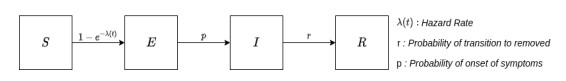
    Related Papers:

    [1] Longfei Wei, Lu Liu, Jialong Hou . Pricing hybrid-triggered catastrophe bonds based on copula-EVT model. Quantitative Finance and Economics, 2022, 6(2): 223-243. doi: 10.3934/QFE.2022010
    [2] Lianzhang Bao, Guangliang Zhao, Zhuo Jin . A new equilibrium trading model with asymmetric information. Quantitative Finance and Economics, 2018, 2(1): 217-229. doi: 10.3934/QFE.2018.1.217
    [3] Manuela Larguinho, José Carlos Dias, Carlos A. Braumann . Pricing and hedging bond options and sinking-fund bonds under the CIR model. Quantitative Finance and Economics, 2022, 6(1): 1-34. doi: 10.3934/QFE.2022001
    [4] Jie Xiong, Geng Deng, Xindong Wang . Extension of SABR Libor Market Model to handle negative interest rates. Quantitative Finance and Economics, 2020, 4(1): 148-171. doi: 10.3934/QFE.2020007
    [5] Lichao Tao, Yuefu Lai, Yanting Ji, Xiangxing Tao . Asian option pricing under sub-fractional vasicek model. Quantitative Finance and Economics, 2023, 7(3): 403-419. doi: 10.3934/QFE.2023020
    [6] Richard J. Cebula, Don Capener . The impact of federal income tax rate cuts on the municipal bond market in the U.S.: A brief exploratory empirical note. Quantitative Finance and Economics, 2018, 2(2): 407-412. doi: 10.3934/QFE.2018.2.407
    [7] Serçin ŞAHİN, Serkan ÇİÇEK . Interest rate pass-through in Turkey during the period of unconventional interest rate corridor. Quantitative Finance and Economics, 2018, 2(4): 837-859. doi: 10.3934/QFE.2018.4.837
    [8] Guillermo Peña . Interest rates affect public expenditure growth. Quantitative Finance and Economics, 2023, 7(4): 622-645. doi: 10.3934/QFE.2023030
    [9] Bonang N. Seoela . Efficacy of monetary policy in a currency union? Evidence from Southern Africa's Common Monetary Area. Quantitative Finance and Economics, 2022, 6(1): 35-53. doi: 10.3934/QFE.2022002
    [10] Mustafa Tevfik Kartal, Özer Depren, Serpil Kılıç Depren . The determinants of main stock exchange index changes in emerging countries: evidence from Turkey in COVID-19 pandemic age. Quantitative Finance and Economics, 2020, 4(4): 526-541. doi: 10.3934/QFE.2020025
  • The ongoing COVID-19 pandemic highlights the essential role of mathematical models in understanding the spread of the virus along with a quantifiable and science-based prediction of the impact of various mitigation measures. Numerous types of models have been employed with various levels of success. This leads to the question of what kind of a mathematical model is most appropriate for a given situation. We consider two widely used types of models: equation-based models (such as standard compartmental epidemiological models) and agent-based models. We assess their performance by modeling the spread of COVID-19 on the Hawaiian island of Oahu under different scenarios. We show that when it comes to information crucial to decision making, both models produce very similar results. At the same time, the two types of models exhibit very different characteristics when considering their computational and conceptual complexity. Consequently, we conclude that choosing the model should be mostly guided by available computational and human resources.


    1. Introduction


    1.1. Background

    In global financial markets, the pricing of a bond becomes more complicated due to different credit rating and different interest rate. A change of credit rating or a change of interest rate may cause drastic swing of bond prices. To manage the complication, one needs to understand how the credit risk impacts on the bond markets and how it can be measured. There are two types of credit risks: defaults and credit rating migrations. In the previous researches, the defaults are paid more attentions. However, in the financial crisis in 2008 and European debt crisis in 2010, the credit rating migrations played a much more important role in the finance and economics than what people expected. Therefore, the study of credit rating migrations becomes significant. Another observed factor in a financial market is that bond prices strongly depend on the interest rate. This leads to a crucial question of how to price a corporate bond with credit rating migration risks and interest rate change.


    1.2. Literature review

    There are many existing research papers on bond pricing models, see examples, Briys and de Varenne (Briys and Varenne, 1997), Tsiveriotis and Fernandes (Tsiveriotis and Fernandes, 1998).To measure default risks, there are two basic frameworks: a structure model, and a reduced form one. It is well-known that the first structure model for credit default proposed by Merton (Merton, 1974) is under the assumption that the firm's value follows a geometric Brownian motion process and the corporate bonds are considered as contingent claims. The default event may only occur at the maturity of the claim. In 1976, Black and Cox extended Merton's model to a first-passage-time model by introducing safety covenants. This extends the original model which gives bondholders the right to recognize a firm's value if its asset falls below some exogenously given threshold. In the modified model(Black and Cox, 1976), the default is allowed to occur any time up to the debt's maturity. By the reduced form framework, the credit events are considered to be governed by exogenous reason stochastically, see (Duffie and Singleton, 1999; Jarrow and Turnbull, 1995; Lando, 1998; Leland and Toft, 1996).

    In study of credit rating migration, a major tool is the Markov chain. Most researchers mainly adopted a transfer intensity matrix. By this approach, the reduced form framework is naturally developed for the dynamic process of credit rating migrations, see Jarrow et al. (1997), Das and Tufano (1996), Hurd and Kuznetsov (2007), Lando (1998), Thomas et al. (2002) and so forth. The transfer intensity matrix usually comes from general statistical data, which do not include any particulary firm's information. However, a firm's own value plays a key role of its credit rating migration. In this situation, the Markov chain alone cannot fully capture the credit-rating mitigation for a firm. From the existing literatures, few research took this into account. Liang et al. (2015) in 2015 used a structure model for pricing bonds with credit rating migrations at first time. They gave a predetermined migration threshold where a firm's value is divided into high and low rating regions, under the assumption that the value of the firm follows a stochastic process. By using Feynman-Kac theorem, these models can be reduced to certain boundary value problems of partial differential equations. This PDE method is very different from the traditional approaches in the research field of corporative bond modelling. However, the rating migration boundary is usually not predetermined in the real financial world. It depends on the proportion of the debt and the value of the firm. From this point of view, the migration boundary should be a free boundary. Recently, Hu et al. (2015) and liang et al. (2016) proposed a new model to reflect this fact under the fixed-interest rate. They obtained the existence and uniqueness for the free boundary problem. Also, they proved that there is a travelling wave in the problem.

    For pricing a bond, interest rate is a sensitive factor. Many stochastic models are used for the model, see Longstarff and Schwartz (1995) as an example. However, when a stochastic interest rate is considered, the bond model becomes two dimensions, which is much harder to analyze.


    1.3. Result description

    So far, all valuations for credit rating migration via pricing a corporate bond by structure model are assumed a constant interest rate. However, the stochastic interest rate for a bond is essential. So the extension for the model to stochastic interest rate is necessary. However, the extension meets a great difficult that the original free boundary model from one dimension to a higher one. That is the main contribution and solved problem in this paper.

    In the present paper, we follow the ideas from (Hu et al., 2015) to derive a new model for a bond price in which credit-rating may change and the interest rate follows a stochastic process. To be more precise, we assume that the interest rate follows a Vasicek's stochastic process and the bond price follows a geometric Brownian motion with a different volatility in different credit-rating region. A coupled system of PDEs is derived. By employing a dimension-reduction technique we are able to simplify the coupled system to a single equation with a nonlinear jump coefficient in the leading term of the equation. Under certain conditions, the existence and uniqueness are established for the new model. We would like to indicate that our approach is different from that in (Hu et al., 2015; Liang et al., 2016). Moreover, the uniqueness proof in Section 4 is new to our knowledge. The method is also suitable for n-dimensional problems. Furthermore, the regularity of the free boundary is also considered. By transforming the problem to a Stefan-like problem, we prove that the free boundary is smooth. Some numerical results are also illustrated in the present paper. Those numerical results are well matching the theoretical analysis.


    1.4. Paper structure

    The paper is organized as follows: In Section 2, a new model with credit-rating migration and stochastic interest rate is rigorously derived under usual assumptions. In Section 3, we use the dimension reduction technique to simplify the model to a free boundary problem. In Section 4, we first use various PDE techniques to derive uniform estimates for the approximate problem. The existence and uniqueness are then established by using a compactness argument. Uniqueness is proved via an energy method. In Section 5, further properties of the solution are shown. In Section 6, some numerical results are presented. Some concluding remarks are given in section 7.


    2. The Derivation of the Model


    2.1. Basic assumptions

    Let (Ω,F,P) be a complete probability space. We assume that the firm issues a corporate bond, which is a contingent claim of its value on the space F.

    Assumption 2.1. Interest rate rt follows Vasicek process:

    drt=a(t)(θ(t)rt)dt+σr(t)dWrt,

    where a(t), θ(t) and σr(t) are given positive functions, which are supposed to be positive constants a,θ,σr for the simplification in this paper. Wrt is the Brownian motion which generates the filtration {Ft}.

    We would like to point out that our model is a big improvement from the assumption of a constant interest rate to the stochastic one. There are many stochastic models for the interest rate, Vesicek model is popular one. The advantage point of this model is simply and easily calculable, while the weak point is the possibility of negative interest rate, which is proved to be very low. We assume that the interest rate follows Vesicek model also because that in our dimension reducing technique, only Vesicek model works.

    Assumption 2.2 (the firm asset with credit rating migration). Let St denote the firm's value in the risk neutral world. It satisfies

    dSt={rtStdt+σH(t)StdWt,inhighratingregion,rtStdt+σL(t)StdWt,inlowratingregion,

    where rt is the risk free interest rate, and

    σH(t)<σL(t) (1)

    represent volatilities of the firm under the high and low credit grades, respectively. They are assumed to be deterministic and differentiable on [0,T] and have a positive lower bound:

    0<˜σ0σH(t)<σL(t)˜σ1<,0tT. (2)

    Wt is the Brownian motion which generates the filtration {Ft}, and

    Cov(dWt,dWrt)=ρdt,

    where 1<ρ<1 is a constant.

    It is reasonable to assume (1), namely, that the volatility in high rating region is lower than the one in the low rating region. This implies that there is a jump for the volatility when the rating changes.

    Assumption 2.3 (the corporate bond). The firm issues only one corporate zero-coupon bond with face value F. Denote Φt the discount value of the bond at time t, which is also the function of rt. Therefore, on the maturity time T, an investor can get ΦT=min{ST,F}.

    Assumption 2.4 (the credit rating migration time). High and low rating regions are determined by the proportion of the debt and value. The credit rating migration time τ1 and τ2 are the first moments when the firm's grade is downgraded and upgraded, respectively, as follows:

    τ1=inf{t>0|Φ0/S0<γ,Φt/Stγ},τ2=inf{t>0|Φ0/S0>γ,Φt/Stγ},

    where Φt=Φt(St,r,t) is a contingent claim with respect to St and

    0<γ<1 (3)

    is a positive constant representing the threshold proportion of the debt and value of the firm's rating.


    2.2. Cash flow

    Once the credit rating migrates before the maturity T, a virtual substitute termination happens, i.e., the bond is virtually terminated and substituted by a new one with a new credit rating. There is a virtual cash flow of the bond. Denoted by ΦH(y,r,t) and ΦL(y,r,t) the values of the bond in high and low grades respectively. Then, they are the conditional expectations as follows:

    ΦH(y,r,t)=Ey,t[eTtrsdsmin(ST,F)1τ1T+eτ1trsdsΦL(Sτ1,rt,τ1)1t<τ1<T|St=y>1γΦH(y,t),rt=r], (4)
    ΦL(y,r,t)=Ey,t[eTtrsdsmin(ST,F)1τ2T+eτ2trsdsΦH(Sτ2,rt,τ2)1t<τ2<T|St=y<1γΦL(y,t),rt=r], (5)

    where 1event={1, if "event" happens ,0, otherwise. 


    2.3. Mathematical model

    By Feynman-Kac formula (Dixit and Pindyck, 1994), it is not difficult to drive that ΦH and ΦL are the function of the firm value S, interest rate r and time t. They satisfy the following partial differential equations in their regions:

    ΦHt+12σ2HS22ΦHS2+σrσHρS2ΦHSr+12σ2r2ΦHr2+rSΦHS+a(θr)ΦHrrΦH=0,S>1γΦH,0<t<T, (6)
    ΦLt+12σ2LS22ΦLS2+σrσLρS2ΦLSr+12σ2r2ΦLr2+rSΦLS+a(θr)ΦLrrΦL=0,S<1γΦL,0<t<T, (7)

    with the terminal condition:

    ΦH(S,T)=ΦL(S,T)=min{S,F}. (8)

    (4) and (5) imply that the value of the bond is continuous when it passes the rating threshold, i.e.,

    ΦH=ΦL=γSon the rating migration boundary. (9)

    Also, as in (Hu et al., 2015; Jin et al., 2016), we have

    ΦHS=ΦLSon the rating migration boundary. (10)

    This is a two-dimensional free boundary problem of an terminate value parabolic problem with discontinuous leading coefficient.


    3. A PDE Problem


    3.1. Reduction of dimension

    The equations (6) and (7) are two-dimensional. For the purpose of simplifying the problem, we could use a technique to reduce the dimension.

    Denote P(rt,t:T) to be the value of a zero-coupon bond faced 1 at time T. So that, it satisfies

    Pt+12σ2r2Pr2+a(θr)PrrP=0, (11)

    which admits a unique solution (Hall, 1989)

    P(r,t:T)=A(t)erB(t), (12)

    where

    A(t)=e{1a2[B2(t)(Tt)](a2θσ2r2)σ24aB2(t)},B(t)=1a(1ea(Tt)).

    Now make a transform by

    y=SP(r,t;T),VH(y,t)=ΦH(S,r,t)P(r,t;T),VL(y,t)=ΦL(S,r,t)P(r,t;T).

    Then V(y,t) satisfies

    VHt+12ˆσ2Hy22VHy2=0,y>1γVH, 0<t<T, (13)
    VLt+12ˆσ2Ly22VLy2=0,y<1γVL, 0<t<T, (14)
    VH(y,T)=VL(y,T)=min{y,F}, (15)

    where

    ˆσi=σ2i+2ρσiσrB(t)+σ2rB2(t),i=H,L. (16)

    And on credit rating migration boundary, there holds

    VH(y,t)=VL(y,t)=γy,VHy=VLy. (17)

    3.2. A free boundary problem

    Using the standard change of variables x=logy and renaming Tt as t, and defining

    ϕ(x,t)={VH(ex,Tt) in high rating region,VL(ex,Tt) in low rating region,

    using also (6) and (7), we then derive the following equation from (6), (7):

    ϕt12σ22ϕx2+12σ2ϕx=0,(x,t)QTΓT (18)

    where

    QT=(,+)×(0,T],ΓT={(x,t)|ϕ(x,t)=γex} (19)

    and σ is a function of ϕ and (x,t), i.e.,

    σ=σ(ϕ,x,t)={ˆσHifϕ<γex,ˆσLifϕγex. (20)

    The constant γ is defined in (3), and ˆσH,ˆσL are defined in (16). There exist constants σ0,σ1, such that

    0<σ0ˆσH,ˆσLσ1<. (21)

    Without loss of generality, we assume F=1. Equation (18) is supplemented with the initial condition (derived from (8))

    ϕ(x,0)=ϕ0(x)=min{ex,1},<x<. (22)

    The domain will be divided into the high rating region QHT where ϕ<γex and a low rating region QLT where ϕ>γex. We shall prove that these two domains will be separated by a free boundary x=s(t), and

    QHT={x>s(t),0<t<T},QLT={x<s(t),0<t<T}. (23)

    In another word, s(t) is apriorily unknown since it should be the solved by the equation

    ϕ(s(t),t)=γes(t),

    where the solution ϕ is apriorily unknown.


    4. Existence and Uniqueness


    4.1. Approximation

    Let H(ξ) be the Heaviside function, i.e., H(ξ)=0 for ξ<0 and H(ξ)=1 for ξ>0. Then we can rewrite (20) as

    σ(t,ϕ)=ˆσH+(ˆσLˆσH)H(ϕγex).

    We use a standard approximation for H(ξ) and ϕ0(x) such that

    Hε(ξ)C(R1)andHε(ξ)=H(ξ)for|ξ|ε,ϕ0ε(x)C3(R1)W1,(R1),ϕ0ε(x)γex<0,for0<x<ln1γ.

    Now we consider the following approximated problem

    ϕεt12σ2ε(2ϕεx2ϕεx)=0,(x,t)QT, (24)
    ϕε(x,0)=ϕ0ε(x),<x<, (25)

    where

    σε=ˆσH+(ˆσLˆσH)Hε(ϕεγex). (26)

    4.2. Estimates

    Lemma 4.1. The problem (24)-(25) admits a unique solution

    ϕε(x,t)C2,1(QT)Cα,α2(¯QT),forforallα(0,1)

    Moreover, the following estimates hold uniformly with respect to ε:

    a) 0ϕε(x,t)1, 0ϕεx(x,t)C1

    b) sup0tT+ϕ2εxdx+QT(ϕ2εxx+ϕ2εt)dxdtC2

    where C1 and C2 depend only on known data.

    Proof. By the theory of parabolic equation, we know that the problem (24)-(25) admits a unique classic solution ϕεC2,1(QT)Cα,α2(¯QT).

    Now we derive the uniform estimates. First of all, by the maximum principle for Cauchy problem, we see

    0ϕε(x,t)1,(x,t)¯QT.

    Let ψε(x,t)=ϕεx(x,t), then

    ψεtx[12σ2ε(ψεxψε)],(x,t)¯QT,ψε(x,0)=ϕ0ε(x)0,<x<+

    Again, since ϕ0ε(x)0, by maximum principle, we obtain

    ψε(x,t)0.

    On the other hand,

    ψεtx(12σ2εψεx)=x(12σ2εψε) (27)

    We multiply equation (27) ψpε for any p1, to obtain

    ddt1p+1+ψp+1εdx+p+12σ2εψ2εxψp1εdx=p+12σ2εψpεψεxdxδ+p12σ2εψp1εψ2εxdx+C(δ)p+12σ2εψp+1εdx.

    If we choose δ sufficiently small, we have

    ddt1p+1+ψp+1εdx+12p+12σ2εψ2εxψp1εdxC+12σ2εψp+1εdx

    Since 0<σ0σεσ1<+, we have

    +ψp+1εdx++t0ψ2εxψp1εdxdt+ϕ0ε(x)2dx+Ct0+ψp+1εdxdt

    Gronwall's inequality yields,

    +ψp+1εdx++T0ψ2εxψp1εdxdtC,

    where C depends only on known data and p, but not on ε.

    Now from equation (27),

    ψεtx(12σ2εψεx)=x(12σ2εψε),(x,t)QTψε(x,0)=ϕ0ε(x),<x<+

    where σ2εψεLp(R1) for any p>1. Then ||ψε||L(QT)C. To derive the W2,12(QT)estimate, we multiply equation (24) by ϕεxx and integrate over Qt to obtain

    σ0Qtϕ2εxxdxdt++ϕ2εxdx+ϕ2εx(x,0)dx=Qt12σ2εϕεxϕεxxdxdtδQtϕ2εxxdxdt+C(δ)Qtϕ2εxdxdt

    By choosing δ sufficiently small, we have

    σ0Qtϕ2εxxdxdt++ϕ2εx(x,t)dx+ϕ2εx(x,0)dx+CQtϕ2εxdxdt

    Gronwall's inequality yields

    sup0tT+ϕ2εxdx+Qtϕ2εxxdxdtC.

    From the equation (24), we see

    Qtϕ2εtdxdtC

    Lemma 4.2. The solution ϕε(x,t)C1+α,1+α2(QT) uniformly with respect to ε, for some α(0,1). Moreover, for any ρ>0 there exists a constant C(ρ) such that

    ||ψε||Cα,α2(ˉQTBρ(0,0))C(ρ),

    where Bρ(0,0)={(x,t):ρ<x<ρ,0<t<ρ} and C(ρ) depends only on known data and ρ.

    Proof. Indeed, we see ψε(x,t) is a solution of the following problem:

    ψεtx[12σ2(ψεxψε)]=0,(x,t)QT,ψε(x,0)=ϕε0(x)0,<x<+.

    By the standard theory for parabolic equations, we see that ψε(x,t) is Hölder continuous in QT. Moreover, the Hölder continuity of ψε holds up to the initial time t=0 except a neighborhood of the singular point (0,0). Hence, for any ρ>0, we have

    ||ψε||Cα,α2(ˉQTBρ(0,0))C(ρ),

    where Bρ(0,0) defined above and C(ρ) depends only on known data and ρ, but not on ε.


    4.3. Existence

    Theorem 4.1. The problem (17), (21) admits a solution ϕ(x,t)W1,0(QT)W2,12(QT)Cα,α2(¯QT), for any α(0,1). Furthermore, the solution satisfies

    a) 0ϕ(x,t)1, 0ϕx(x,t)C1,

    b) +ϕ2xdx+QT(ϕ2xx+ϕ2t)dxdtC2,

    where C1 and C2 are constants which depend only on known data.

    Proof. By the standard compactness argument, we see that there exists a function ϕ(x,t)Cα,α2(¯QT)W2,12(QT) such that

    ϕε(x,t)ϕ(x,t)uniformly in Cα,α2(¯QT),ϕε(x,t)ϕ(x,t)weakly in W2,12(QT).

    Moreover, 0ϕ(x,t)1, 0ϕx(x,t)C1. For the limit function ϕ, and (x0,t0) with (x0,t0)ΓT and t0>0, where ΓT is defined in (19), there exists a small neighborhood Pδ(x0,t0)={(x,t)|(xx0)2+(tt0)2<δ} such that Pδ(x0,t0)ΓT=. In Pδ(x0,t0), σε(x,t,ϕ)=σ(x,t,ϕ). By regularity theory of parabolic equation, ϕ(x,t)C2,1(Pδ(x0,t0)), and

    ϕt12σ2(ϕxxϕx)=0.

    It follows that for any (x,t)ΓT

    ϕt12σ2(ϕxxϕx)=0,in the classical sense in QTΓT,ϕ(x,0)=ϕ0(x),<x<+.

    Notice also by Lemma 4.2, ϕ,ϕx are continuous across ΓT. That is, ϕ(x,t) is a solution in QT.

    We can obtain a better regularity for the strong solution obtained in Theorem 4.1.

    Theorem 4.2. The solution ϕ(x,t)C1+α,1+α2(QT) for some α(0,1). Moreover, ϕx(x,t) is Hölder continuous up to the initial time t=0 except a neighborhood of (0,0).

    Proof. Indeed, we see ψ(x,t)=ϕx(x,t) is a weak solution of the following problem:

    ψt=x[12σ2(ψxψ)],(x,t)QT,ψ(x,0)=ϕ0(x)0,<x<+.

    By the standard regularity theory of parabolic equations, we see that ψ(x,t) is Hölder continuous in QT. Moreover, the Hölder continuity of ψ holds up to the initial time t=0 except a neighborhood of the singular point (0,0).


    4.4. Uniqueness

    In this section we use a novel approach to prove the uniqueness. This method is also suitable for a general n-dimensional problem.

    Theorem 4.3. The solution obtained in Theorem 4.1 is unique.

    Proof. We rewrite Eq.(18) as follows:

    k(ϕ,x,t)ϕt=ϕxxϕx, (28)

    where

    k(ϕ,x,t)={2/ˆσ2L(t), if ϕ>γex,2/ˆσ2H(t), if ϕ<γex.

    Define

    e(ϕ,x,t)=(1/ˆσ2L(t)+1/ˆσ2H(t))(ϕγex)+(1/ˆσ2L(t)1/ˆσ2H(t))|ϕγex|={2(ϕγex)/ˆσ2L(t), if ϕ>γex,2(ϕγex)/ˆσ2H(t), if ϕ<γex. (29)

    which satisfies that

    k(ϕ,x,t)=eϕ={2/ˆσ2L(t), if ϕ>γex,2/ˆσ2H(t), if ϕ<γex. (30)

    Therefore,

    t[e(ϕ,x,t)][ϕxxϕx]=etf(ϕ,x,t), (31)

    where

    f(ϕ,x,t):=(1/ˆσ2L(t)+1/ˆσ2H(t))(ϕγex)+(1/ˆσ2L(t)1/ˆσ2H(t))|ϕγex|.

    We also have

    e(ϕ,x,t)|t=0=e0(x), (32)

    where

    e0(x)=(1/ˆσ2L(0)+1/ˆσ2H(0))(ϕ0(x)γex)+(1/ˆσ2L(0)1/ˆσ2H(0))|ϕ0(x)γex|,

    To prove the uniqueness, we assume that there are two solutions ϕi(x,t), i=1,2 of the problem (17), (21), which satisfy the estimates in Theorem 4.1. Set

    ϕ(x,t)=ϕ1(x,t)ϕ2(x,t),(x,t)QT.

    Now we multiply τtϕ(x,s)ds in the both sides of (31), where τ[0,T], and then integrate it in R, we have

    tR[(e(ϕ1,x,t)e(ϕ2,x,t))τtϕds]dx+R[(e(ϕ1,x,t)e(ϕ2,x,t))ϕ]dx=R[(ϕxxϕx)τtϕds]dx+R[(f(ϕ1,x,t)f(ϕ2,x,t))τtϕds]dx:=A1(x,t,τ)+A2(x,t,τ),

    where

    A1(t,τ)=R[(ϕxxϕx)τtϕds]dx,A2(t,τ)=R[(f(ϕ1,x,t)f(ϕ2,x,t))τtϕds]dx.

    Now,

    A1(t,τ)=R[(ϕxϕ)τtϕxds]dx=12tR[τtϕxds]2dx+R[ϕτtϕxds]dx.
    A2(t,τ)=R[(fϕ(ξ,t)ϕ)τtϕds]dx,

    where ξ is the mean-value between ϕ1 and ϕ2.

    We take integration to the above equation with respect to t from 0 to τ to obtain:

    τ0R[e(ϕ1,x,t)e(ϕ2,x,t)]ϕdxdt+12R[τ0ϕxds]2dx=τ0R+[ϕτtϕxds]dxdt+τ0R(fϕ(ξ,x,t)ϕ)τtϕdsdxdt2ετ0Rϕ2dxdt+C(ε)τ0R([τ0ϕds]2+[τ0ϕxds]2)dxdt.

    Here at the final step we have used the uniform boundedness of fu(u,t) and Cauchy-Schwarz's inequality with small parameter ε.

    Notice (29), we have

    [e(ϕ1,x,t)e(ϕ2,x,t)]c0(ϕ1ϕ2)=(2/σ21)ϕ,

    where σ1 defined in (21) has a positive lower bound. We choose ε sufficiently small to obtain

    τ0Rϕ2dxdt+R[τ0ϕxds]2dxC[τ0[t0Rϕ2dxds]dt+τ0R[τ0ϕxds]2dxdt].

    Consequently, Gronwall's inequality yields ϕ(x,t)0 on Qτ. As τ is arbitrary over [0,T], we have ϕ(x,t)0 on QT.

    Thin concludes the proof of uniqueness.


    5. Free Boundary and its Regularity

    In this section, we show that ΓT is the graph of a smooth free boundary x=s(t).

    Lemma 5.1. There exists a number T0>0, such that ΓT0 defined in (19) is the graph of a function x=s(t),0tT0 with s(0)=s0=ln1γ.

    Proof. Note that ϕ0(x)=min{ex,1}, then s0:=s(0)=ln1/γ>0, it follows that ϕ0(x)=0, for x>0; ϕ0(x)=ex, for x<0. It follows that if x>0,

    ϕ0(x)γex=γex<0.

    Since ϕx(x,t) is Hölder continuous except (0,0), there exists small numbers t0>0 and δ0>0 such that

    ϕx(x,t)γexm0<0,s0δ0<x<s0+δ0,0tt0,

    where m0 depends on t0 and δ0.

    By the implicit function theorem, there exists a function, denoted by x=s(t) solves ϕ(s(t),t)=γes(t) such that

    Γt0={(x,t)|x=s(t),0tt0}.

    It will be seen in the next theorem that we can extend t0 as long as ϕx(s(t),t)γes(t)<0.

    Theorem 5.1. There exists a function x=s(t)Cβ[0,T] with β(12,1) such that

    ΓT={(s(t),t):0tT}.

    Moreover, there exists a constant ε0>0 such that

    ϕx(s(t),t)γes(t)ε0<0,0tT.

    Proof. From Lemma 5.1, we know that there exists at least a small internal [0,T0] such that

    ΓT0={(s(t),t):0tT0.}

    Moreover,

    ϕx(s(t),t)γes(t)<0,t[0,T0].

    Since F(x,t):=ϕ(x,t)γex is differentiable in QT with respect to x, by the implicit function theorem, the set

    Γt0={(x,t);F(x,t)=0,0tt0}

    can be extended as the graph of a curve x=s(t) as long as

    Fx(x,t)<0,for all (x,t)ΓT.

    Moreover, x=s(t) is decreasing on [0,T].

    Define

    T=sup{T0:ϕx(s(t),t)γes(t)<0,0tT0}.

    We claim T=T. Assume the contrary with T<T. It is clear by the definition of T and the continuity of ϕx(x,t) that

    limtT(ϕx(s(t),t)γes(t))=0.

    We define W(x,t)=ϕ(x,t)γex, then

    Wt=ϕt,Wx=ϕxγex,Wxx=ϕxxγex

    Therefore, W(x,t) satisfies

    Wt12σ2H(WxxWx)=0,<x<s(t),0<t<T,W(s(t),t)=0,0<t<T,W(x,0)=W0(x),<x<s0,

    where W0(x):=ϕ0(x)γex0 on (,s0].

    Since s(t) is decreasing on [0,T), Hopf's lemma holds at (s(T),T). Hence, by Hopf's lemma, there exists a number ε0>0 such that Wx(s(T),T)ε0<0, which contradicts with the definition of T. It follows that T=T. Consequently, there exists a curve, denoted by x=s(t), such that

    ΓT={(s(t),t):0tT.}.

    Moreover, there exists a constant ε0>0 such that

    ϕx(s(t),t)γes(t)ε0<0,0tT. (33)

    To prove the Hölder continuity of s(t) on [0,T], we take any t1<t2 in [0,T] with |t1t2| sufficiently small,

    ϕ(s(t2),t2)ϕ(s(t1),t1)=γ(es(t2)es(t1)).

    Then,

    ϕ(s(t2),t1)ϕ(s(t1),t1)γ(es(t2)es(t1))=ϕ(s(t2),t1)ϕ(s(t2),t2).

    We use the mean-value theorem to obtain

    |s(t2)s(t1)||ϕ(s(t2),t2)ϕ(s(t2),t1)||Fx(θ,t1)|,

    where θ is the mean-value between s(t1) and s(t2).

    Since |Fx(x,t)| is bounded and |Fx(x,t)| has a positive lower bound in a neighborhood of x=s(t),0tT, we find that there exists a constant C such that

    |s(t2)s(t1)|C|t1t2|β,

    where β=1+α2.

    It follows that s(t) is Hölder continuous on [0,T] with a Hölder exponent β(12,1).

    Theorem 5.2. The free boundary s(t) satisfies

    s(t)=σH(t)(ϕxx(s(t),t)ϕx(s(t),t))ϕx(s(t),t)γes(t),0tT.

    Moreover, s(t)C[0,T], provided that σL(t) and σH(t) are smooth on [0,T].

    Proof. By Theorem 5.1, we can define QLT and QHT as in Section 3. From the theory of parabolic equations (Ladyženskaja et al., 1968), we know that ϕ(x,t) is smooth in QLT and QHT, respectively. Moreover, ϕx(x,t) is continuous up the boundary x=s(t) from the left-hand side and the right-hand side on [0,T].

    To prove the further regularity of s(t), we note that ψ(x,t)=ϕx(x,t) is a classical solution of the following free boundary problem

    ψt=x[12σ2(ψxxψ)],(x,t)QTΓT,ψ(s(t),t)=ψ(s(t)+,t),0<t<T,σH(ψx(s(t),t)ψ(s(t),t))=σL(ψx(s(t)+,t)ψ(s(t)+,t)),0tT,s(t)=σH(t)(ψx(s(t),t)ψ(s(t),t))ψ(s(t),t)γes(t),0tT,ψ(x,0)=ϕ0(x),<x<.

    We can apply the classical technique for the Musket problem Evans (1978) to obtain s(t)C[0,].

    Theorem 5.3. s(t) is non-increasing on [0.T].

    Proof. We go back the approximate problem (24)-(25). Note that ϕ0(x)ϕ0(x)=0 if x<0 and ϕ0(x)ϕ0(x)=1 if x>0. We can construct a smooth approximation for ϕ0(x) such that

    ϕε0ϕ0(x)<0,<x<.

    Let w(x,t)=ϕεt(x,t). Then w(x,t) satisfies

    wt=12σ2[wxxwx]+a(x,t)w,(x,t)QT.

    where

    a(x,t):=(σ2(t,ϕ))tσ2(t,ϕ).

    Moreover,

    w(x,0)=12σε(0,ϕ0)2[ϕ0ε(x)ϕ0ε(x)]<0,<x<.

    By the maximum principle, we see w(x,t)0 on QT. After passing the limit, we see

    ϕxx(x,t)ϕx(x,t)0,(x,t)QT,

    in the L2-sense. On the other hand,

    ϕx(s(t),t)γes(t)<0,0tT,

    we see from the representation of s(t) that

    s(t)0,t[0,T].

    6. Numerical Example

    The numerical solution of the Eq.(17), (21) can be calculated by using a standard PDE method. However, we are more interested in the. For convenience, the free boundary is denoted by s(r,t), which depends on the interest rate r.

    In order to draw the graph s(r,t), we use the explicit difference scheme (Jiang, 2005), which is equivalent to the well-known the Binomial-Tree method. The steps of the computation are as follows:

    1. Discrete t(0,T) by ti=TiΔt, where T=t0,...,tI=0, I=10, Δt=tIt0I; r(0.01,0.04) by rk=0.01+kΔr, where 0.01=r0,...,rK=0.04, Δr=rKr0K; in space using a mesh with difference Δx: 0=x0,...,xj=2. And at every point (ti,xj,rk), denote the function ϕ(ti,xj,rk) by ϕi,j,k.

    2. For t0=T, ϕ0,j,k=min(xj,F), then solve ϕi,j,k by finite difference scheme:

    ϕi,j,k=ϕi1,j,k+σ2Δt2Δx2x2j[ϕi1,j1,k+ϕi1,j+1,k2ϕi1,j,k]+σ2rΔt2Δr2r2k[ϕi1,j,k1+ϕi1,j,k+12ϕi1,j,k]+rkxjΔt2Δx[ϕi1,j+1,kϕi1,j1,k]+a(θrk)Δt2Δr[ϕi1,j,k+1ϕi1,j,k1]rkϕi1,j,kΔt+σσrΔtρxj4ΔrΔx[ϕi1,j+1,k+11ϕi1,j+1,k1ϕi1,j1,k+1+ϕi1,j1,k1],

    where

    σ={σL, if ϕi1,j,k>γxk,σH, otherwise, 

    Denote the joint points to be sj,k, which represents the approximated credit rating migration joints.

    3. Repeat the above process.

    4. Draw the graph based on {sj,k} in space r.S,t.

    Now we have the 2-d free boundary interface.

    The numerical solution of the free boundary is shown in Figure 1, where the parameters and the ranges of the variables are chosen as follows

    a=1,θ=0.03,F=1,γ=0.8,σL=0.4,σH=0.2,σr=0.3,ρ=0.5,T=5,r(0.01,0.04), t(0,5).
    Figure 1. The credit rating migration surface (free boundary) s(r,t).

    From the graphs, we see that a free boundary y=s(r,t) divides the region into two parts: high and low rating regions. Moreover, the free boundary is decreasing with respect to r and increasing with respect to t as expected (see Theorem 4.1 and Theorem 5.2), where t is the original life time of the bond. From the graph Fig. 1, we also see that the change of free boundary is more sensitive with respect to the interest rate than that of time.


    7. Conclusion

    In this paper, we derived a new model for pricing corporate bonds with credit-rating migration and a stochastic interest rate. The new model consists of a coupled system of partial differential equations. By employing a dimension-deduction technique, we obtain a new free boundary problem. By using various analysis techniques for partial differential equations, we established the existence, uniqueness and regularities of the solution under certain assumptions. Moreover, some properties of the solution are derived. A C-regularity of the free boundary is proved. Their financial implications are explained. The model is new to our knowledge and is a big improvement for the current model. The analysis is delicate. Finally, numerical simulations are also presented.


    Acknowledgement

    This work is supported by National Natural Science Foundation of China (No.11671301).The authors would like to thank Professor Bei Hu for some discussions during the preparation of the paper. Many thanks also go to anonymous referees for their comments and suggestions. Chen and Yin would like to thank the hospitalities of Tongji University during their visiting where the part of this work was completed.


    Conflict of Interest

    All authors declare no conflicts of interest in this paper.


    [1] Modelling a pandemic with asymptomatic patients, impact of lockdown and herd immunity, with applications to SARS-CoV-2. Annu Rev Control (2020) 50: 432-447.
    [2]

    J. Balisacan, M. Chyba and C. Shanbrom, Two new compartmental epidemiological models and their equilibria, COVID-19 SARS-CoV-2 Preprints from MedRxiv and BioRxiv, (2021).

    [3]

    C. Branas et al., Flattening the curve before it flattens us: hospital critical care capacity limits and mortality from novel coronavirus (SARS-CoV2) cases in US counties, medRxiv, (2020).

    [4]

    M. G. Burch, K. A. Jacobsen, J. H. Tien and G. A. Rempala, Network-based analysis of a small ebola outbreak, Math. Biosci. Eng., 14 (2017), 67–77, arXiv: 1511.02362.

    [5]

    S. Cauchemez et al., Role of Social Networks in Shaping Disease Transmission During a Community Outbreak of 2009 H1N1 Pandemic Influenza, Proceedings of the National Academy of Sciences, 108 (2011), 2825–2830.

    [6]

    Center for Infectious Disease Research and Policy, Coroner: First US COVID-19 death occurred in early February, https://www.cidrap.umn.edu/news-perspective/2020/04/coroner-first-us-covid-19-death-occurred-early-february.

    [7]

    Centers for Disease Control and Prevention, Emergence of SARS-CoV-2 B.1.1.7 Lineage-United States, December 29, 2020-January 12, 2021, Morbidity and Mortality Weekly Report (MMWR), 70 (2021), 95–99, https://www.cdc.gov/mmwr/volumes/70/wr/mm7003e2.htm.

    [8] Understanding the metropolis-hastings algorithm. The american statistician (1995) 49: 327-335.
    [9]

    M. Chyba, Y. Mileyko, O. Markovichenko, R. Carney and A. Koniges, Epidemiological model of the spread of COVID-19 in Hawai'is chanllenging fight against the didease, The Ninth International Conference on Global Health Challenges, Proceedings, (2020), 32–38.

    [10] Analysis of an SEIRS epidemic model with two Delays. J. Math. Biol. (1990) 35: 240-258.
    [11] An agent-based model to evaluate the COVID-19 transmission risks in facilities. Comput Biol Med (2020) 121: 103827.
    [12] Mathematical models of contact patterns between age groups for predicting the spread of infectious diseases. Mathematical Biosciences and Engineering (2013) 10: 1475-1497.
    [13]

    N. M. Ferguson et al., Report 9 - Impact of non-pharmaceutical interventions (NPIs) to reduce COVID-19 mortality and healthcare demand, MRC Centre for Global Infectious Disease Analysis, Imperial College, (2020).

    [14]

    M. Gatto et al., Spread and dynamics of the COVID-19 epidemic in Italy: Effects of emergency containment measures, Proceedings of the National Academy of Sciences, (2020).

    [15]

    G. Giordano et al., Modelling the COVID-19 epidemic and implementation of population-wide interventions in Italy, Nature Medicine, (2020).

    [16] A network-based analysis of the 1861 hagelloch measles data. Biometrics (2012) 68: 755-765.
    [17]

    W. T. Harvey et al., SARS-CoV-2 variants, spike mutations and immune escape, Nature Reviews Microbiology, 19 (2021), 409–424.

    [18]

    Hawaii Department of Health COVID Dashboard, https://health.hawaii.gov/coronavirusdisease2019/what-you-should-know/current-situation-in-hawaii/.

    [19]

    Hawaii Population Model. Hawai'i Data Collaborative, https://www.hawaiidata.org/hawaii-population-model, (2021).

    [20]

    Hawaii Safe Travels Digital Platform, https://hawaiicovid19.com/travel/data/.

    [21]

    E. M. Hendrix, et al., Introduction to Nonlinear and Global Optimization, Springer Optimization and Its Applications, 37. Springer, New York, 2010.

    [22] Three basic epidemiological models. Applied Mathematical Ecology (Trieste, 1986) (1989) 18: 119-144.
    [23] The mathematics of infectious diseases. SIAM Review (2000) 42: 599-653.
    [24]

    Z. Jin et al., Modelling and analysis of influenza A (H1N1) on networks, BMC public health, 11 (2011), 1–9.

    [25]

    D. G. Kendall, Deterministic and stochastic epidemics in closed populations, Proceedings of the Third Berkeley Symposium on Mathematical Statistics and Probability, 1954-1955, (1956), 149–165.

    [26] Contributions to the mathematical theory of epidemics. Ⅱ.-The problem of endemicity. Proceedings of the Royal Society of London. Series A, containing papers of a mathematical and physical character (1932) 138: 55-83.
    [27] A contribution to the mathematical theory of epidemics. R. Soc. Lond. A (1927) 115: 700-721.
    [28]

    C. C. Kerr et al., Covasim: An agent-based model of COVID-19 dynamics and interventions, medRxiv, (2020).

    [29] Global stability of a SEIR epidemic model with vertical transmission. SIAM J. Appl.Math. (2001) 62: 58-69.
    [30] Curtailing transmission of severe acute respiratory syndrome within a community and its hospital. Royal Society (2003) 270: 1979-1989.
    [31]

    E. Mathieu, H. Ritchie and E. Ortiz-Ospina, et al., Coronavirus (COVID-19) Vaccinations, A Global Database of COVID-19 Vaccinations. Nat Hum Behav, (2021), https://ourworldindata.org/covid-vaccinations.

    [32]

    L. H. Nguye et al., Risk of COVID-19 among front-line health-care workers and the general community: A prospective cohort study, The Lancet Public Health, 5 (2020), e475–e483.

    [33]

    Ö. Ozme et al., Analyzing the impact of modeling choices and assumptions in compartmental epidemiological models, Simulation (SAGE journals), 92 (2016), 459–472.

    [34] A systematic review of covid-19 epidemiology based on current evidence. J. Clin. Med. (2020) 9: 967.
    [35]

    K. Prem et al., The effect of control strategies to reduce social mixing on outcomes of the COVID-19 epidemic in Wuhan, China: a modelling study, The Lancet Public Health, 5 (2020), e261–e270.

    [36] Management strategies in a SEIR-type model of COVID 19 community spread. Sci Rep (2020) 10: 21256.
    [37]

    C. W. Reynolds, Flocks, herds and schools: A distributed behavioral model, Seminal Graphics: Pioneering Efforts that Shaped the Field, (1998), 273–282.

    [38] A network model for ebola spreading. Elsevier (2016) 394: 212-222.
    [39] An Application of the Theory of Probabilities to the Study of a priori Pathometry. Part Ⅰ. Proceedings of the Royal Society of London Series A (1916) 92: 204-230.
    [40] An application of the theory of probabilities to the study of a priori pathometry. Part Ⅱ. Proceedings of the Royal Society of London Series A (1917) 93: 212-225.
    [41]

    G. Sabetian et al., COVID-19 infection among healthcare workers: A cross-sectional study in southwest Iran, Virology Journal, 18 (2021), 58.

    [42] Dynamic models of segregation. The Journal of Mathematical Sociology (1971) 1: 143-186.
    [43]

    T. C. Schelling, Micromotives and Macrobehavior, WW Norton & Company, 1978.

    [44]

    The New York Times, New Coronavirus Cases in U.S. Soar Past 68,000, Shattering Record, https://www.nytimes.com/2020/07/10/world/coronavirus-updates.html.

    [45]

    The New York Times, The U.S. Now Leads the World in Confirmed Coronavirus Cases, https://www.nytimes.com/2020/03/26/health/usa-coronavirus-cases.html.

    [46]

    A. Truszkowska et al., High-resolution agent-based modeling of COVID-19 spreading in a small town, Advanced Theory and Simulations, 4 (2021), 2000277.

    [47]

    World Health Organization, Listings of WHO's response to COVID-19, https://www.who.int/news/item/29-06-2020-covidtimeline.

    [48]

    F. Zhou, et al., Clinical course and risk factors for mortality of adult inpatients with COVID-19 in Wuhan, China: a retrospective cohort study, The Lancet, (2020).

  • This article has been cited by:

    1. Zhehao Huang, Tianpei Jiang, Zhenzhen Wang, On a multiple credit rating migration model with stochastic interest rate, 2020, 43, 0170-4214, 7106, 10.1002/mma.6435
    2. Hong-Ming Yin, Jin Liang, Yuan Wu, On a New Corporate Bond Pricing Model with Potential Credit Rating Change and Stochastic Interest Rate, 2018, 11, 1911-8074, 87, 10.3390/jrfm11040087
    3. Shilong Li, Xia Zhao, Chuancun Yin, Zhiyue Huang, Stochastic interest model driven by compound Poisson process and Brownian motion with applications in life contingencies, 2018, 2, 2573-0134, 246, 10.3934/QFE.2018.1.246
    4. Juri Kandilarov, Lubin Vulkov, 2019, Chapter 47, 978-3-030-10691-1, 416, 10.1007/978-3-030-10692-8_47
    5. Shilong Li, Xia Zhao, Chuancun Yin, Zhiyue Huang, Stochastic interest model driven by compound Poisson process and Brownian motion with applications in life contingencies, 2018, 2, 2573-0134, 731, 10.3934/QFE.2018.1.731
    6. Zhehao Huang, Zhenghui Li, Zhenzhen Wang, Utility Indifference Valuation for Defaultable Corporate Bond with Credit Rating Migration, 2020, 8, 2227-7390, 2033, 10.3390/math8112033
    7. Stephanie Heck, Corporate bond yields and returns: a survey, 2022, 36, 1934-4554, 179, 10.1007/s11408-021-00394-4
    8. Jin Liang, Yang Lin, A traveling wave with a buffer zone for asymptotic behavior of an asymmetric fixed credit migration model, 2022, 0170-4214, 10.1002/mma.8974
    9. Zhongdi Cen, Jian Huang, Aimin Xu, Anbo Le, An iterative method for solving a PDE with free boundary arising from pricing corporate bond with credit rating migration, 2023, 8, 2473-6988, 3286, 10.3934/math.2023169
    10. Xinfu Chen, Jin Liang, A Free Boundary Problem for Corporate Bond Pricing and Credit Rating Under Different Upgrade and Downgrade Thresholds, 2021, 12, 1945-497X, 941, 10.1137/20M1343592
    11. Chen Xinfu, Hu Bei, Liang Jin, Yin Hongming, The free boundary problem for measuring credit rating migration risks, 2023, 1674-7216, 10.1360/SSM-2022-0151
    12. Jin Liang, Yang Lin, A Bond Pricing Model with Credit Migration Risk: Different Upgrade and Downgrade Thresholds, 2023, 39, 0168-9673, 765, 10.1007/s10255-023-1082-3
    13. Yuchao Dong, Jin Liang, Claude-Michel Brauner, Double free boundary problem for defaultable corporate bond with credit rating migration risks and their asymptotic behaviors, 2023, 372, 00220396, 505, 10.1016/j.jde.2023.06.050
    14. Xinfu Chen, Jin Liang, Variational inequalities arising from credit rating migration with buffer zone, 2023, 0956-7925, 1, 10.1017/S095679252300030X
    15. Yang Lin, Jin Liang, A Multi-Credit-Rating Migration Model with Asymmetric Migration Boundaries, 2024, 29, 2297-8747, 7, 10.3390/mca29010007
    16. Jin Liang, Bei Hu, 2024, Chapter 6, 978-981-97-2178-8, 109, 10.1007/978-981-97-2179-5_6
    17. Jin Liang, Bei Hu, 2024, Chapter 8, 978-981-97-2178-8, 167, 10.1007/978-981-97-2179-5_8
    18. Alicia Vidler, Toby Walsh, 2025, Decoding OTC Government Bond Market Liquidity: An ABM Model for Market Dynamics, 979-8-3315-0831-9, 1, 10.1109/CiFer64978.2025.10975734
  • Reader Comments
  • © 2022 the Author(s), licensee AIMS Press. This is an open access article distributed under the terms of the Creative Commons Attribution License (http://creativecommons.org/licenses/by/4.0)
通讯作者: 陈斌, bchen63@163.com
  • 1. 

    沈阳化工大学材料科学与工程学院 沈阳 110142

  1. 本站搜索
  2. 百度学术搜索
  3. 万方数据库搜索
  4. CNKI搜索

Metrics

Article views(1656) PDF downloads(186) Cited by(7)

Article outline

Figures and Tables

Figures(17)  /  Tables(5)

/

DownLoad:  Full-Size Img  PowerPoint
Return
Return

Catalog