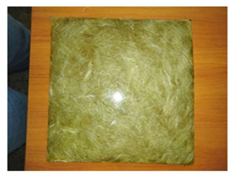
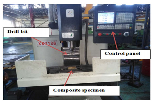
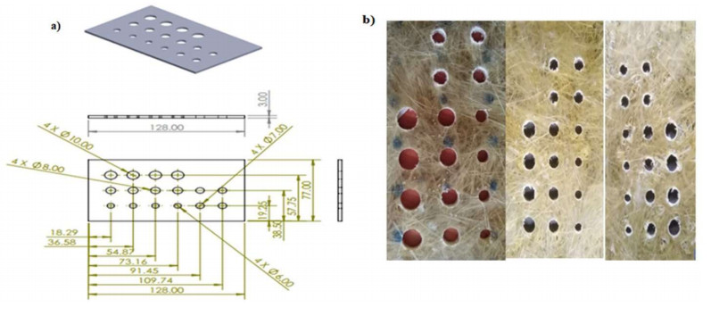
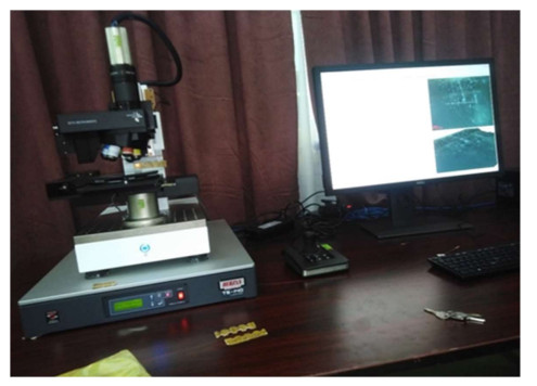
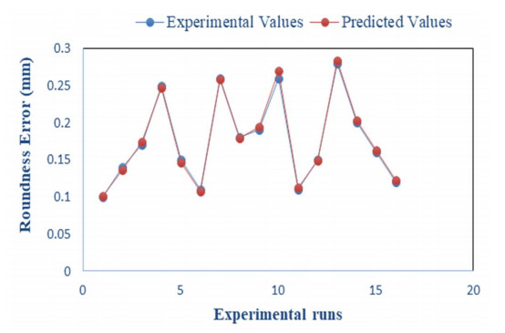
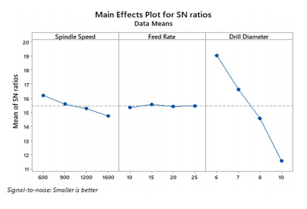
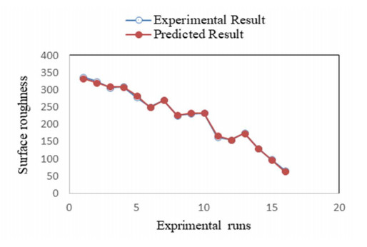
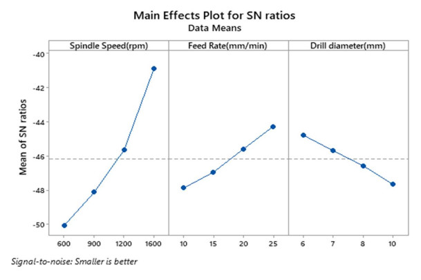
Machining natural fiber reinforced polymer composite materials is one of most challenging tasks due to the material's anisotropic property, non-homogeneous structure and abrasive nature of fibers. Commonly, conventional machining of composites leads to delamination, inter-laminar cracks, fiber pull out, poor surface finish and wear of cutting tool. However, these challenges can be significantly reduced by using proper machining conditions. Thus, this research aims at optimizing machining parameters in drilling hybrid sisal-cotton fibers reinforced polyester composite for better machining performance characteristics namely better hole roundness accuracy and surface finish using Taguchi method. The effect of machining parameters including spindle speed, feed rate and drill diameter on drill hole accuracy (roundness error) and surface-roughness of the hybrid composite are evaluated. Series of experiments based on Taguchi's L16 orthogonal array were performed using different ranges of machining parameters namely spindle speed (600,900, 1200, 1600 rpm), feed rate (10, 15, 20, 25 mm/min) and drill diameter (6, 7, 8, 10 mm). Hole roundness error and surface-roughness are determined using ABC digital caliper and Zeta 20 profilometer, respectively. Optimum machining condition for drilling hybrid composite material (speed: 1600 rpm, feed rate: 25 mm/min and drill diameter: 6 mm) is determined, and the results are verified by conducting confirmation test which proves that the results are reliable.
Citation: Nurhusien Hassen Mohammed, Desalegn Wogaso Wolla. Optimization of machining parameters in drilling hybrid sisal-cotton fiber reinforced polyester composites[J]. AIMS Materials Science, 2022, 9(1): 119-134. doi: 10.3934/matersci.2022008
Machining natural fiber reinforced polymer composite materials is one of most challenging tasks due to the material's anisotropic property, non-homogeneous structure and abrasive nature of fibers. Commonly, conventional machining of composites leads to delamination, inter-laminar cracks, fiber pull out, poor surface finish and wear of cutting tool. However, these challenges can be significantly reduced by using proper machining conditions. Thus, this research aims at optimizing machining parameters in drilling hybrid sisal-cotton fibers reinforced polyester composite for better machining performance characteristics namely better hole roundness accuracy and surface finish using Taguchi method. The effect of machining parameters including spindle speed, feed rate and drill diameter on drill hole accuracy (roundness error) and surface-roughness of the hybrid composite are evaluated. Series of experiments based on Taguchi's L16 orthogonal array were performed using different ranges of machining parameters namely spindle speed (600,900, 1200, 1600 rpm), feed rate (10, 15, 20, 25 mm/min) and drill diameter (6, 7, 8, 10 mm). Hole roundness error and surface-roughness are determined using ABC digital caliper and Zeta 20 profilometer, respectively. Optimum machining condition for drilling hybrid composite material (speed: 1600 rpm, feed rate: 25 mm/min and drill diameter: 6 mm) is determined, and the results are verified by conducting confirmation test which proves that the results are reliable.

| [1] | UD Din I, Hao P, Aamir M, et al. (2019) FEM implementation of the coupled elastoplastic/damage model: Failure prediction of fiber reinforced polymers FRPs composites. J Solid Mech 11: 842–853. |
| [2] |
Aamir M, Tolouei-Rad M, Giasin K, et al. (2019) Recent advances in drilling of carbon fiber reinforced polymers for aerospace applications: A review. J Adv Manuf Technol 105: 2289–2308. https://doi.org/10.1007/s00170-019-04348-z doi: 10.1007/s00170-019-04348-z

|
| [3] | Davim PJ (2010) Machining Composites Materials, London: Wiley & Sons. https://doi.org/10.1002/9781118602713 |
| [4] |
Hassan A, Khan R, Khan N, et al. (2021) Effect of seawater ageing on fracture toughness of stitched glass fiber/epoxy laminates for marine applications. J Mar Sci Eng 196: 1–9. https://doi.org/10.3390/jmse9020196 doi: 10.3390/jmse9020196
|
| [5] |
Guen-Geffroy L, Davies P, Le Gac PY, et al. (2020) Influence of seawater ageing on fracture of carbon fiber reinforced epoxy composites for ocean engineering. Oceans 1: 198–214. https://doi.org/10.3390/oceans1040015 doi: 10.3390/oceans1040015
|
| [6] |
Boscato G, Mottram JT, Russo S (2011) Dynamic response of a sheet pile of fiber-reinforced polymer for waterfront barriers. J Compos Constr 15: 974–984. https://doi.org/10.1061/(ASCE)CC.1943-5614.0000231 doi: 10.1061/(ASCE)CC.1943-5614.0000231
|
| [7] |
Rubino F, Nisticò A, Tucci F, et al. (2020) Marine application of fiber reinforced composites: A review. J Mar Sci Eng 8: 1–26. https://doi.org/10.3390/jmse8010026 doi: 10.3390/jmse8010026
|
| [8] |
Srinivasakumar P, Nandan MJ, Kiran CU, et al. (2013) Sisal and its potential for creating innovative employment opportunities and economic prospects. IOSR J Mech Civ Eng 8: 1–8. https://doi.org/10.9790/1684-0860108 doi: 10.9790/1684-0860108
|
| [9] | Kalia S, Kaith BS, Kaur I (2011). Cellulose Fibers: Bio-and Nano-Polymer Composites: Green Chemistry and Technology, Berlin: Springer. https://doi.org/10.1007/978-3-642-17370-7 |
| [10] | Hufenbach W, Dobrzański LA, Gude M, et al. (2007) Optimization of the rivet joints of the CFRP composite material and aluminium alloy. J Achiev Mater Manuf Eng 20: 119–122. |
| [11] |
Teti R (2002) Machining of composite materials. Cirp Ann Manuf Techn 51: 611–634. https://doi.org/10.1016/S0007-8506(07)61703-X doi: 10.1016/S0007-8506(07)61703-X
|
| [12] |
Mirsha R, Malik J, Singh I, et al. (2010) Neural network approach for estimate the residual tensile strength after drilling in unidirectional glass fiber reinforced plastic laminates. Mater Design 31: 2790–2795. https://doi.org/10.1016/j.matdes.2010.01.011 doi: 10.1016/j.matdes.2010.01.011
|
| [13] |
Abrão AM, Faria PE, Campos Rubio JC, et al. (2007) Drilling of fiber reinforced plastics: A review. J Mater Process Tech 186: 1–7. https://doi.org/10.1016/j.jmatprotec.2006.11.146 doi: 10.1016/j.jmatprotec.2006.11.146
|
| [14] |
Liu D, Tang Y, Cong W (2012) A review of mechanical drilling for composite laminates. Compos Struct 94: 1265–1279. https://doi.org/10.1016/j.compstruct.2011.11.024 doi: 10.1016/j.compstruct.2011.11.024
|
| [15] | Dinesh G, Guru Moorthy A, Balaji AN, Mechanical and corrosion properties of hybrid sisal fibre/cotton fibre/coconut sheath reinforced polymer composites, 2019. Available from: https://www.mzcet.in/naac/documents/cf91.pdf. |
| [16] |
Kurt M, Bagci E, Kaynak Y (2009) Application of Taguchi methods in the optimization of cutting parameters for surface finish and hole diameter accuracy in dry drilling processes. Int J Adv Manuf Tech 40: 458–469. https://doi.org/10.1007/s00170-007-1368-2 doi: 10.1007/s00170-007-1368-2
|
| [17] |
Davim JP, Reis P (2003) Drilling carbon fiber reinforced plastic manufactured by auto clave experimental and statistical study. Mater Design 24: 315–324. https://doi.org/10.1016/S0261-3069(03)00062-1 doi: 10.1016/S0261-3069(03)00062-1
|
| [18] | Korkut I, Kucuk Y (2010) Experimental analysis of the deviation from circularity of bored hole based on the Taguchi method. Stroj Vestn-J Mech E 56: 340–346. |
| [19] |
Tsao CC, Hocheng H (2008) Evaluation of thrust force and surface roughness in drilling composite material using Taguchi analysis and neural network. J Mater Process Tech 203: 342–348. https://doi.org/10.1016/j.jmatprotec.2006.04.126 doi: 10.1016/j.jmatprotec.2006.04.126
|
| [20] |
Sahoo P, Barman TK, Routara BC (2008) Fractal dimension modelling of surface profile and optimization in CNC end milling using response surface method. Int J Manuf Res 3: 360–377. https://doi.org/10.1504/IJMR.2008.019216 doi: 10.1504/IJMR.2008.019216
|
| [21] |
Hadi RM, Mohsen H, Masatoshi K, et al. (2019) Experimental study on drilling of jute fiber reinforced polymer composites. J Compos Mater 53: 283–295. https://doi.org/10.1177/0021998318782376 doi: 10.1177/0021998318782376
|
| [22] | Taguchi G, Konishi S (1987) Taguchi Methods, Orthogonal Arrays and Linear Graphs: Tools for Quality Engineering, Dearborn Michigan: American Supplier Institute, 35–38. |
| [23] |
Rao RS, Kumar CG, Prakasham RS, et al. (2008) The Taguchi methodology as a statistical tool for biotechnological application: A critical appraisal. Biotechnol J 3: 510–523. https://doi.org/10.1002/biot.200700201 doi: 10.1002/biot.200700201
|
| [24] | Yang WP, Tarng Y (1998) Design optimization of cutting parameters for turning operations based on the Taguchi method. J Mater Process Tech 84: 122–129. https://doi.org/10.1016/S0924-0136(98)00079-X |
| [25] |
Lotfi A, Li H, Dao DV (2019) Machinability analysis in drilling flax fiber-reinforced polylactic acid bio-composite laminates. Int J Mater Metall Eng 13: 443–447. https://doi.org/10.5281/zenodo.3455743 doi: 10.5281/zenodo.3455743
|
| [26] | Philip JR (1996) Taguchi Techniques for Quality Engineering: Loss Function, Orthogonal Experiments, Parameter and Tolerance Design, 2 Eds., Chennai: McGraw-Hill Education (India) Private Limited. |
| [27] | Phadke MS (1989) Quality engineering using robust design, London: Prentice-Hall, 07632. https://doi.org/10.1007/978-1-4684-1472-1_3 |
| [28] |
Ravishankar B, Nayak SK, Kader MA (2019) Hybrid composites for automotive applications–A review. J Reinf Plast Comp 38: 835–845. https://doi.org/10.1177/0731684419849708 doi: 10.1177/0731684419849708
|
| [29] |
Al-Oqla FM, Sapuan SM (2014) Natural fiber reinforced polymer composites in industrial applications: Feasibility of date palm fibers for sustainable automotive industry. J Clean Prod 66: 347–354. https://doi.org/10.1016/j.jclepro.2013.10.050 doi: 10.1016/j.jclepro.2013.10.050
|
Figures(8) / Tables(9)

Nurhusien Hassen Mohammed, Desalegn Wogaso Wolla. Optimization of machining parameters in drilling hybrid sisal-cotton fiber reinforced polyester composites[J]. AIMS Materials Science, 2022, 9(1): 119-134. doi: 10.3934/matersci.2022008


 DownLoad: