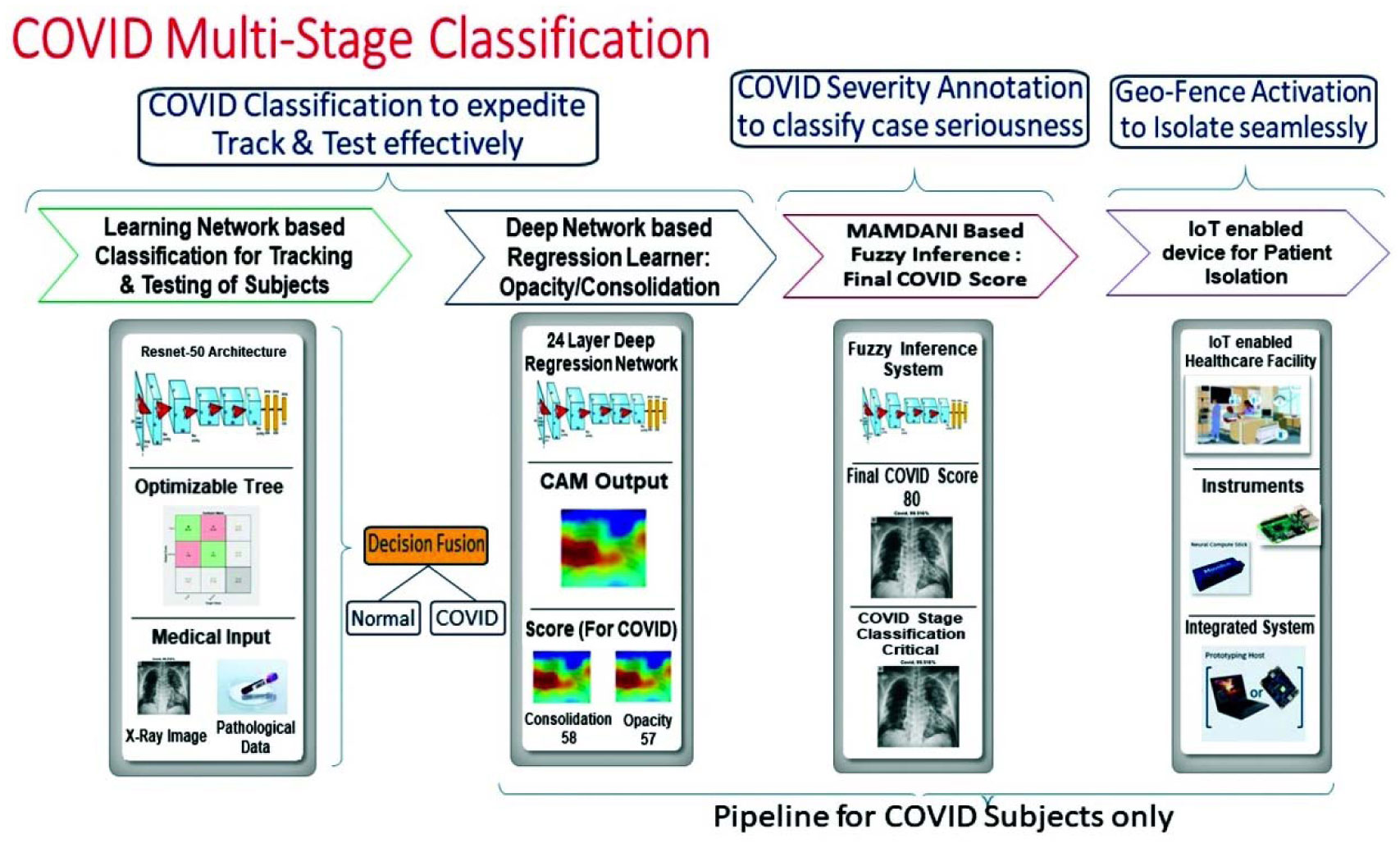
The use of Artificial Intelligence (AI) in combination with Internet of Things (IoT) drastically reduces the need to test the COVID samples manually, saving not only time but money and ultimately lives. In this paper, the authors have proposed a novel methodology to identify the COVID-19 patients with an annotated stage to enable the medical staff to manually activate a geo-fence around the subject thus ensuring early detection and isolation. The use of radiography images with pathology data used for COVID-19 identification forms the first-ever contribution by any research group globally. The novelty lies in the correct stage classification of COVID-19 subjects as well. The present analysis would bring this AI Model on the edge to make the facility an IoT-enabled unit. The developed system has been compared and extensively verified thoroughly with those of clinical observations. The significance of radiography imaging for detecting and identification of COVID-19 subjects with severity score tag for stage classification is mathematically established. In a Nutshell, this entire algorithmic workflow can be used not only for predictive analytics but also for prescriptive analytics to complete the entire pipeline from the diagnostic viewpoint of a doctor. As a matter of fact, the authors have used a supervised based learning approach aided by a multiple hypothesis based decision fusion based technique to increase the overall system's accuracy and prediction. The end to end value chain has been put under an IoT based ecosystem to leverage the combined power of AI and IoT to not only detect but also to isolate the coronavirus affected individuals. To emphasize further, the developed AI model predicts the respective categories of a coronavirus affected patients and the IoT system helps the point of care facilities to isolate and prescribe the need of hospitalization for the COVID patients.
Citation: Swarnava Biswas, Debajit Sen, Dinesh Bhatia, Pranjal Phukan, Moumita Mukherjee. Chest X-Ray image and pathological data based artificial intelligence enabled dual diagnostic method for multi-stage classification of COVID-19 patients[J]. AIMS Biophysics, 2021, 8(4): 346-371. doi: 10.3934/biophy.2021028
The use of Artificial Intelligence (AI) in combination with Internet of Things (IoT) drastically reduces the need to test the COVID samples manually, saving not only time but money and ultimately lives. In this paper, the authors have proposed a novel methodology to identify the COVID-19 patients with an annotated stage to enable the medical staff to manually activate a geo-fence around the subject thus ensuring early detection and isolation. The use of radiography images with pathology data used for COVID-19 identification forms the first-ever contribution by any research group globally. The novelty lies in the correct stage classification of COVID-19 subjects as well. The present analysis would bring this AI Model on the edge to make the facility an IoT-enabled unit. The developed system has been compared and extensively verified thoroughly with those of clinical observations. The significance of radiography imaging for detecting and identification of COVID-19 subjects with severity score tag for stage classification is mathematically established. In a Nutshell, this entire algorithmic workflow can be used not only for predictive analytics but also for prescriptive analytics to complete the entire pipeline from the diagnostic viewpoint of a doctor. As a matter of fact, the authors have used a supervised based learning approach aided by a multiple hypothesis based decision fusion based technique to increase the overall system's accuracy and prediction. The end to end value chain has been put under an IoT based ecosystem to leverage the combined power of AI and IoT to not only detect but also to isolate the coronavirus affected individuals. To emphasize further, the developed AI model predicts the respective categories of a coronavirus affected patients and the IoT system helps the point of care facilities to isolate and prescribe the need of hospitalization for the COVID patients.

| [1] |
Sun T, Wang Y (2020) Modeling COVID-19 epidemic in Heilongjiang province, China. Chaos, Soliton Fract 138: 109949. doi: 10.1016/j.chaos.2020.109949

|
| [2] |
Melin P, Castillo O (2021) Spatial and temporal spread of the COVID-19 pandemic using self organizing neural networks and a fuzzy fractal approach. Sustainability 13: 8295. doi: 10.3390/su13158295
|
| [3] |
Castillo O, Melin P (2021) A novel method for a covid-19 classification of countries based on an intelligent fuzzy fractal approach. Healthcare 9: 196. doi: 10.3390/healthcare9020196
|
| [4] |
Castillo O, Melin P (2020) Forecasting of COVID-19 time series for countries in the world based on a hybrid approach combining the fractal dimension and fuzzy logic. Chaos, Soliton Fract 140: 110242. doi: 10.1016/j.chaos.2020.110242
|
| [5] |
Boccaletti S, Ditto W, Mindlin G, et al. (2020) Modeling and forecasting of epidemic spreading: The case of Covid-19 and beyond. Chaos, Soliton Fract 135: 109794. doi: 10.1016/j.chaos.2020.109794
|
| [6] | Wang W, Xu Y, Gao R, et al. (2020) Detection of SARS-CoV-2 in different types of clinical specimens. Jama 323: 1843-1844. |
| [7] | West CP, Montori VM, Sampathkumar P (2020) COVID-19 testing: the threat of false-negative results. Elsevier 95: 1127-1129. |
| [8] |
Fang Y, Zhang H, Xie J, et al. (2020) Sensitivity of chest CT for COVID-19: comparison to RT-PCR. Radiology 296: E115-E117. doi: 10.1148/radiol.2020200432
|
| [9] |
Ng M-Y, Lee EY, Yang J, et al. (2020) Imaging profile of the COVID-19 infection: radiologic findings and literature review. Radiolo: Cardiothorac Imag 2: e200034. doi: 10.1148/ryct.2020200034
|
| [10] |
Huang C, Wang Y, Li X, et al. (2020) Clinical features of patients infected with 2019 novel coronavirus in Wuhan, China. The lancet 395: 497-506. doi: 10.1016/S0140-6736(20)30183-5
|
| [11] |
Guan WJ, Ni ZY, Hu Y, et al. (2020) Clinical characteristics of coronavirus disease 2019 in China. New Engl J Med 382: 1708-1720. doi: 10.1056/NEJMoa2002032
|
| [12] |
Ai T, Yang Z, Hou H, et al. (2020) Correlation of chest CT and RT-PCR testing for coronavirus disease 2019 (COVID-19) in China: a report of 1014 cases. Radiology 296: E32-E40. doi: 10.1148/radiol.2020200642
|
| [13] |
Khatami F, Saatchi M, Zadeh SST, et al. (2020) A meta-analysis of accuracy and sensitivity of chest CT and RT-PCR in COVID-19 diagnosis. Sci Rep 10: 22402. doi: 10.1038/s41598-020-80061-2
|
| [14] |
Nair A, Rodrigues JCL, Hare S, et al. (2020) A British society of thoracic imaging statement: considerations in designing local imaging diagnostic algorithms for the COVID-19 pandemic. Clin Radiol 75: 329-334. doi: 10.1016/j.crad.2020.03.008
|
| [15] |
Jacobi A, Chung M, Bernheim A, et al. (2020) Portable chest X-ray in coronavirus disease-19 (COVID-19): A pictorial review. Clin Imag 64: 35-42. doi: 10.1016/j.clinimag.2020.04.001
|
| [16] | LeCun Y, Bengio Y, Hinton G (2015) Deep learning. Nature . |
| [17] | Gozes O, Frid-Adar M, Greenspan H, et al. Rapid ai development cycle for the coronavirus (covid-19) pandemic: Initial results for automated detection & patient monitoring using deep learning ct image analysis (2020) .arXiv preprint arXiv:2003.05037. |
| [18] | Lessmann N, Sánchez CI, Beenen L, et al. (2020) Automated assessment of CO-RADS and chest CT severity scores in patients with suspected COVID-19 using artificial intelligence. Radiology . |
| [19] | Li L, Qin L, Xu Z, et al. (2020) Artificial intelligence distinguishes COVID-19 from community acquired pneumonia on chest CT. Radiology . |
| [20] |
Shi F, Xia L, Shan F, et al. (2021) Large-scale screening to distinguish between COVID-19 and community-acquired pneumonia using infection size-aware classification. Phys Med Biol 66: 065031. doi: 10.1088/1361-6560/abe838
|
| [21] | Magree H, Russell F, Sa'Aga R, et al. (2005) Chest X-ray-confirmed pneumonia in children in Fiji. B World Health Organ 83: 427-433. |
| [22] |
Wong HYF, Lam HYS, Fong AHT, et al. (2020) Frequency and distribution of chest radiographic findings in patients positive for COVID-19. Radiology 296: E72-E78. doi: 10.1148/radiol.2020201160
|
| [23] |
Borghesi A, Maroldi R (2020) COVID-19 outbreak in Italy: experimental chest X-ray scoring system for quantifying and monitoring disease progression. La radiologia medica 125: 509-513. doi: 10.1007/s11547-020-01200-3
|
| [24] | Wang X, Peng Y, Lu L, et al. (2017) Chestx-ray8: Hospital-scale chest x-ray database and benchmarks on weakly-supervised classification and localization of common thorax diseases. Proceedings of the IEEE conference on computer vision and pattern recognition 2097-2106. |
| [25] | Rajpurkar P, Irvin J, Zhu K, et al. Chexnet: Radiologist-level pneumonia detection on chest x-rays with deep learning (2017) .arXiv preprint arXiv:1711.05225. |
| [26] |
Wang H, Jia H, Lu L, et al. (2019) Thorax-Net: An attention regularized deep neural network for classification of thoracic diseases on chest radiography. IEEE J Biomed Health 24: 475-485. doi: 10.1109/JBHI.2019.2928369
|
| [27] |
Rajaraman S, Candemir S, Kim I, et al. (2018) Visualization and interpretation of convolutional neural network predictions in detecting pneumonia in pediatric chest radiographs. Appl Sci 8: 1715. doi: 10.3390/app8101715
|
| [28] |
Kermany DS, Goldbaum M, Cai W, et al. (2018) Identifying medical diagnoses and treatable diseases by image-based deep learning. Cell 172: 1122-1131. doi: 10.1016/j.cell.2018.02.010
|
| [29] |
Horry MJ, Chakraborty S, Paul M, et al. (2020) COVID-19 detection through transfer learning using multimodal imaging data. IEEE Access 8: 149808-149824. doi: 10.1109/ACCESS.2020.3016780
|
| [30] | Ahmed I, Ahmad A, Jeon G (2020) An iot based deep learning framework for early assessment of covid-19. IEEE Internet Things J . |
| [31] |
Chowdhury MEH, Rahman T, Khandakar A, et al. (2020) Can AI help in screening viral and COVID-19 pneumonia? IEEE Access 8: 132665-132676. doi: 10.1109/ACCESS.2020.3010287
|
| [32] |
Han Z, Wei B, Hong Y, et al. (2020) Accurate screening of COVID-19 using attention-based deep 3D multiple instance learning. IEEE T Med Imaging 39: 2584-2594. doi: 10.1109/TMI.2020.2996256
|
| [33] |
Qian X, Fu H, Shi W, et al. (2020) M $^ 3$ Lung-Sys: A deep learning system for multi-class lung pneumonia screening from CT imaging. IEEE J Biomed Health 24: 3539-3550. doi: 10.1109/JBHI.2020.3030853
|
| [34] |
Sakib S, Tazrin T, Fouda MM, et al. (2020) DL-CRC: deep learning-based chest radiograph classification for COVID-19 detection: a novel approach. IEEE Access 8: 171575-171589. doi: 10.1109/ACCESS.2020.3025010
|
| [35] |
Waheed A, Goyal M, Gupta D, et al. (2020) Covidgan: data augmentation using auxiliary classifier gan for improved covid-19 detection. Ieee Access 8: 91916-91923. doi: 10.1109/ACCESS.2020.2994762
|
| [36] |
Varela-Santos S, Melin P (2021) A new approach for classifying coronavirus COVID-19 based on its manifestation on chest X-rays using texture features and neural networks. Inform Sci 545: 403-414. doi: 10.1016/j.ins.2020.09.041
|
| [37] |
Brihn A, Chang J, OYong K, et al. (2021) Diagnostic performance of an antigen test with RT-PCR for the detection of SARS-CoV-2 in a hospital setting—Los Angeles county, California, June–August 2020. Morbid Mortal W Rep 70: 702. doi: 10.15585/mmwr.mm7019a3
|
| [38] |
Chawla NV, Bowyer KW, Hall LO, et al. (2002) SMOTE: synthetic minority over-sampling technique. J Artif Intell Res 16: 321-357. doi: 10.1613/jair.953
|
| [39] |
Hassan M, Ali S, Alquhayz H, et al. (2020) Developing intelligent medical image modality classification system using deep transfer learning and LDA. Sci Rep 10: 1-14. doi: 10.1038/s41598-019-56847-4
|
| [40] | He K, Zhang X, Ren S, et al. (2016) Identity mappings in deep residual networks Springer, 630-645. |
| [41] |
Prakash C, Rajkumar S, Mouli PC (2012) Medical image fusion based on redundancy DWT and Mamdani type min-sum mean-of-max techniques with quantitative analysis. 2012 International conference on recent advances in computing and software systems IEEE, 54-59. doi: 10.1109/RACSS.2012.6212697
|
| [42] | Gayathri BM, Sumathi CP (2015) Mamdani fuzzy inference system for breast cancer risk detection. 2015 IEEE International Conference on Computational Intelligence and Computing Research (ICCIC) IEEE, 1-6. |
| [43] | Terrada O, Raihani A, Bouattane O, et al. (2018) Fuzzy cardiovascular diagnosis system using clinical data. 2018 4th International Conference on Optimization and Applications (ICOA) IEEE, 1-4. |
| [44] |
Yang W, Cao Q, Qin LE, et al. (2020) Clinical characteristics and imaging manifestations of the 2019 novel coronavirus disease (COVID-19): a multi-center study in Wenzhou city, Zhejiang, China. J Infection 80: 388-393. doi: 10.1016/j.jinf.2020.02.016
|
| [45] |
Yoon SH, Lee KH, Kim JY, et al. (2020) Chest radiographic and CT findings of the 2019 novel coronavirus disease (COVID-19): analysis of nine patients treated in Korea. Korean J Radiol 21: 494-500. doi: 10.3348/kjr.2020.0132
|
| [46] |
Rodrigues JCL, Hare SS, Edey A, et al. (2020) An update on COVID-19 for the radiologist-A British society of thoracic imaging statement. Clin Radiol 75: 323-325. doi: 10.1016/j.crad.2020.03.003
|
| [47] |
Ludvigsson JF (2020) Systematic review of COVID-19 in children shows milder cases and a better prognosis than adults. Acta Paediatr 109: 1088-1095. doi: 10.1111/apa.15270
|
| [48] |
Holshue ML, DeBolt C, Lindquist S, et al. (2020) First case of 2019 novel coronavirus in the United States. N Engl J Med 382: 929-936. doi: 10.1056/NEJMoa2001191
|
| [49] |
Yang R, Li X, Liu H, et al. (2020) Chest CT severity score: an imaging tool for assessing severe COVID-19. Radiol: Cardiothorac Imag 2: e200047. doi: 10.1148/ryct.2020200047
|
| [50] |
Zhang W, Thurow K, Stoll R (2014) A knowledge-based telemonitoring platform for application in remote healthcare. Int J Comput Commun 9: 644-654. doi: 10.15837/ijccc.2014.5.661
|
| [51] |
Dong J, Zhuang D, Huang Y, et al. (2009) Advances in multi-sensor data fusion: Algorithms and applications. Sensors 9: 7771-7784. doi: 10.3390/s91007771
|
| [52] |
Gevaert CM, García-Haro FJ (2015) A comparison of STARFM and an unmixing-based algorithm for Landsat and MODIS data fusion. Remote Sens Environ 156: 34-44. doi: 10.1016/j.rse.2014.09.012
|
| [53] |
Fourati H (2014) Heterogeneous data fusion algorithm for pedestrian navigation via foot-mounted inertial measurement unit and complementary filter. IEEE T Instrum Meas 64: 221-229. doi: 10.1109/TIM.2014.2335912
|
| [54] |
Ambühl L, Menendez M (2016) Data fusion algorithm for macroscopic fundamental diagram estimation. Transport Res Part C: Emer Technol 71: 184-197. doi: 10.1016/j.trc.2016.07.013
|


Figures(20) / Tables(7)

Swarnava Biswas, Debajit Sen, Dinesh Bhatia, Pranjal Phukan, Moumita Mukherjee. Chest X-Ray image and pathological data based artificial intelligence enabled dual diagnostic method for multi-stage classification of COVID-19 patients[J]. AIMS Biophysics, 2021, 8(4): 346-371. doi: 10.3934/biophy.2021028


 DownLoad: