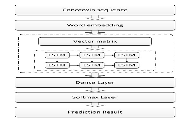
Aiming at the problems of the wet experiment method in identifying the types of conotoxins, such as the complexity, low efficiency and high cost, this study proposes a method that uses the sequence information of the conotoxin peptides combined with long short term memory networks (LSTM) models to predict the Methods of spirotoxin category. This method only needs to take the conotoxin peptide sequence as input, and adopts the character embedding method in text processing to automatically map the sequence to the feature vector representation, and the model extracts features for training and prediction. Experimental results show that the correct index of this method on the test set reaches 0.80, and the AUC value reaches 0.817. For the same test set, the AUC value of the KNN algorithm is 0.641, and the AUC value of the method proposed in this paper is 0.817, indicating that this method can effectively assist in identifying the type of conotoxin.
Citation: Feng Wang, Shan Chang, Dashun Wei. Prediction of conotoxin type based on long short-term memory network[J]. Mathematical Biosciences and Engineering, 2021, 18(5): 6700-6708. doi: 10.3934/mbe.2021332
Aiming at the problems of the wet experiment method in identifying the types of conotoxins, such as the complexity, low efficiency and high cost, this study proposes a method that uses the sequence information of the conotoxin peptides combined with long short term memory networks (LSTM) models to predict the Methods of spirotoxin category. This method only needs to take the conotoxin peptide sequence as input, and adopts the character embedding method in text processing to automatically map the sequence to the feature vector representation, and the model extracts features for training and prediction. Experimental results show that the correct index of this method on the test set reaches 0.80, and the AUC value reaches 0.817. For the same test set, the AUC value of the KNN algorithm is 0.641, and the AUC value of the method proposed in this paper is 0.817, indicating that this method can effectively assist in identifying the type of conotoxin.

| [1] |
J. Thewissen, J. D. Sensor, M. T. Clementz, S. Bajpai, Evolution of dental wear and diet during the origin of whales, Paleobiology, 37 (2011), 655-669. doi: 10.1666/10038.1

|
| [2] |
Z. Li, G. Beauchamp, M. S. Mooring, Relaxed selection for tick-defense grooming in Père David's deer?, Biol. Conserv., 178 (2014), 12-18. doi: 10.1016/j.biocon.2014.06.026
|
| [3] | D. J. Adams, P. F. Alewood, D. J. Craik, R. D. Drinkwater, R. J. Lewis, Conotoxins and their potential pharmaceutical applications, Drug Dev. Res., 46 (2015), 219-234. |
| [4] |
J. P. Johnson, J. R. Balser, P. B. Bennett, A novel extracellular calcium sensing mechanism in voltage-gated potassium ion channels, J. Neurosci., 21 (2001), 4143-4153. doi: 10.1523/JNEUROSCI.21-12-04143.2001
|
| [5] | R. H. Cox, N. J. Rusch, New expression profiles of voltage-gated ion channels in arteries exposed to high blood pressure, Microcirculation, 9 (2015), 243-257. |
| [6] |
M. Verhulsel, M. Vignes, S. Descroix, L. Malaquin, D. M. Vignjevic, J. L. Viovy, A review of microfabrication and hydrogel engineering for micro-organs on chips, Biomaterials, 35 (2014), 1816-1832. doi: 10.1016/j.biomaterials.2013.11.021
|
| [7] |
A. Fu, Z. Zhao, F. Gao, M. Zhang, Cellular uptake mechanism and therapeutic utility of a novel peptide in targeted-delivery of proteins into neuronal cells, Pharm. Res., 30 (2013), 2108-2117. doi: 10.1007/s11095-013-1068-6
|
| [8] |
A. Beyeler, N. Kadiri, S. Navailles, M. B. Boujema, F. Gonon, C. Le Moine, et al., Stimulation of serotonin2C receptors elicits abnormal oral movements by acting on pathways other than the sensorimotor one in the rat basal ganglia, Neuroscience, 169 (2010), 158-170. doi: 10.1016/j.neuroscience.2010.04.061
|
| [9] | O. Wesołowska, Interaction of phenothiazines, stilbenes and flavonoids with multidrug resistance-associated transporters, P-glycoprotein and MRP1, Acta Biochim. Pol., 58 (2011), 433-448. |
| [10] |
Y. Yang, Y. Cai, G. Wu, X. Chen, C. Zeng, Plasma long non-coding RNA, CoroMarker, a novel biomarker for diagnosis of coronary artery disease, Clin. Sci., 129 (2015), 675-685. doi: 10.1042/CS20150121
|
| [11] | R. Mason, Application of cathodoluminescence imaging to the study of sedimentary rocks, J. Geol., 115 (2006), 710-710. |
| [12] |
L. F. Yuan, C. Ding, S. H. Guo, H. Ding, W. Chen, H. Lin, Prediction of the types of ion channel-targeted conotoxins based on radial basis function network, Toxicol. Vitro, 27 (2013), 852-856. doi: 10.1016/j.tiv.2012.12.024
|
| [13] |
S. Jouanneau, L. Reroutes, M. J. Durand, A. Boukabache, V. Picot, Y. Primault, et al., Methods for assessing biochemical oxygen demand (BOD): A review, Water Res., 49 (2014), 62-82. doi: 10.1016/j.watres.2013.10.066
|
| [14] | L. Zhang, C. Zhang, R. Gao, R. Yang, Q. Song, Using the SMOTE technique and hybrid features to predict the types of ion channel-targeted conotoxins, J. Theor. Biol., (2016), 75-84. |
| [15] | J. Wang, R. M. Nishikawa, Y. Yang, Improving the accuracy in detection of clustered microcalcifications with a context-sensitive classification model, Med. Phys., 43 (2016), 159. |
| [16] |
M. L. Pall, Electromagnetic fields act via activation of voltage-gated calcium channels to produce beneficial or adverse effects, J. Cell. Mol. Med., 17 (2013), 958-965. doi: 10.1111/jcmm.12088
|
| [17] |
J. Szendroedi, W. Sandtner, T. Zarrabi, E. Zebedin, K. Hilber, S. C. Dudley, et al., Speeding the recovery from ultraslow inactivation of voltage-gated Na+ channels by metal ion binding to the selectivity filter: a foot-on-the-door?, Biophys. J., 93 (2007), 4209-4224. doi: 10.1529/biophysj.107.104794
|
| [18] | J. Bandyopadhyay, J. Velázquez, Blow-up rate estimates for the solutions of the bosonic Boltzmann-Nordheim equation, J. Math. Phys., 56 (2015), 761-847. |
| [19] |
C. Angulo, F. J. Ruiz, L. González, J. A. Ortega, Multi-classification by using tri-class SVM, Neural Process. Lett., 23 (2006), 89-101. doi: 10.1007/s11063-005-3500-3
|
| [20] |
J. C. Chang, S. G. Hilsenbeck, S. Fuqua, Genomic approaches in the management and treatment of breast cancer, Br. J. Cancer, 92 (2005), 618-624. doi: 10.1038/sj.bjc.6602410
|
| [21] |
J. Yin, L. Tian, Joint confidence region estimation for area under ROC curve and Youden index, Stat. Med., 33 (2014), 985-1000. doi: 10.1002/sim.5992
|
| [22] |
A. Mihret, Y. Bekele, K. Bobosha, M. Kidd, A. Aseffa, R. Howe, et al., Plasma cytokines and chemokines differentiate between active disease and non-active tuberculosis infection, J. Infect., 66 (2013), 357-365. doi: 10.1016/j.jinf.2012.11.005
|
| [23] |
K. Sasaki, H. M. Kantarjian, E. J. Jabbour, S. O'Brien, J. E. Cortes, Clinical application of artificial intelligence in patients with chronic myeloid leukemia in chronic phase, Blood, 128 (2016), 940-940. doi: 10.1182/blood.V128.22.940.940
|


Figures(5) / Tables(1)

Feng Wang, Shan Chang, Dashun Wei. Prediction of conotoxin type based on long short-term memory network[J]. Mathematical Biosciences and Engineering, 2021, 18(5): 6700-6708. doi: 10.3934/mbe.2021332


 DownLoad: