A privacy preserving recommendation and fraud detection method based on graph convolution

Yunfei Tan; Shuyu Li; Zehua Li; Yunfei Tan; Shuyu Li; Zehua Li

doi:10.3934/era.2023382

Electronic Research Archive

2023, Volume 31, Issue 12: 7559-7577. doi: 10.3934/era.2023382

Previous Article Next Article

Research article Special Issues

A privacy preserving recommendation and fraud detection method based on graph convolution

School of Computer Science, Shaanxi Normal University, Xi'an 710119, China

Received: 16 September 2023 Revised: 14 November 2023 Accepted: 17 November 2023 Published: 04 December 2023

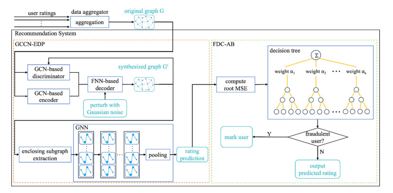
As a typical deep learning technique, Graph Convolutional Networks (GCN) has been successfully applied to the recommendation systems. Aiming at the leakage risk of user privacy and the problem of fraudulent data in the recommendation systems, a Privacy Preserving Recommendation and Fraud Detection method based on Graph Convolution (PPRFD-GC) is proposed in the paper. The PPRFD-GC method adopts encoder/decoder framework to generate the synthesized graph of rating information which satisfies edge differential privacy, next applies graph-based matrix completion technique for rating prediction according to the synthesized graph. After calculating user's Mean Square Error (MSE) of rating prediction and generating dense representation of the user, then a fraud detection classifier based on AdaBoost is presented to identify possible fraudsters. Finally, the loss functions of both rating prediction module and fraud detection module are linearly combined as the overall loss function. The experimental analysis on two real datasets shows that the proposed method has good recommendation accuracy and anti-fraud attack characteristics on the basis of preserving users' link privacy.
- recommendation system,
- graph convolution,
- matrix completion,
- fraud detection,
- differential privacy
Citation: Yunfei Tan, Shuyu Li, Zehua Li. A privacy preserving recommendation and fraud detection method based on graph convolution[J]. Electronic Research Archive, 2023, 31(12): 7559-7577. doi: 10.3934/era.2023382

Related Papers:

Abstract

As a typical deep learning technique, Graph Convolutional Networks (GCN) has been successfully applied to the recommendation systems. Aiming at the leakage risk of user privacy and the problem of fraudulent data in the recommendation systems, a Privacy Preserving Recommendation and Fraud Detection method based on Graph Convolution (PPRFD-GC) is proposed in the paper. The PPRFD-GC method adopts encoder/decoder framework to generate the synthesized graph of rating information which satisfies edge differential privacy, next applies graph-based matrix completion technique for rating prediction according to the synthesized graph. After calculating user's Mean Square Error (MSE) of rating prediction and generating dense representation of the user, then a fraud detection classifier based on AdaBoost is presented to identify possible fraudsters. Finally, the loss functions of both rating prediction module and fraud detection module are linearly combined as the overall loss function. The experimental analysis on two real datasets shows that the proposed method has good recommendation accuracy and anti-fraud attack characteristics on the basis of preserving users' link privacy.

References

[1]	J. Lu, B. Pan, A. M. Seid, B. Li, G. Hu, S. Wan, Truthful incentive mechanism design via internalizing externalities and lp relaxation for vertical federated learning, IEEE Trans. Comput. Social Syst., 2022. https://doi.org/10.1109/TCSS.2022.3227270 doi: 10.1109/TCSS.2022.3227270
[2]	S. Liu, J. Yu, X. Deng, S. Wan, FedCPF: An efficient-communication federated learning approach for vehicular edge computing in 6G communication networks, IEEE Trans. Comput. Social Syst., 23 (2021), 1616–1629. https://doi.org/10.1109/TITS.2021.3099368 doi: 10.1109/TITS.2021.3099368
[3]	C. Wang, C. Jiang, J. Wang, S. Shen, S. Guo, P. Zhang, Blockchain-aided network resource orchestration in intelligent internet of things, IEEE Internet Things J., 10 (2022), 6151–6163. https://doi.org/10.1109/JIOT.2022.3222911 doi: 10.1109/JIOT.2022.3222911
[4]	J. Lu, H. Liu, R. Jia, J. Wang, L. Sun, S. Wan, Towards personalized federated learning via group collaboration in ⅡoT, IEEE Trans. Ind. Inf., 19 (2022), 8923–8932. https://doi.org/10.1109/TⅡ.2022.3223234 doi: 10.1109/TⅡ.2022.3223234
[5]	G. Wu, L. Xie, H. Zhang, J. Wang, S. Shen, S. Yu, STSIR: An individual-group game-based model for disclosing virus spread in Social Internet of Things, J. Network Comput. Appl., 214 (2023), 103608. https://doi.org/10.1016/j.jnca.2023.103608 doi: 10.1016/j.jnca.2023.103608
[6]	S. Shen, L. Xie, Y. Zhang, G. Wu, H. Zhang, S. Yu, Joint differential game and double deep q-networks for suppressing malware spread in industrial internet of things, IEEE Trans. Inf. Forensics Secur., 18 (2023), 5302–5315. https://doi.org/10.1109/TIFS.2023.3307956 doi: 10.1109/TIFS.2023.3307956
[7]	G. Wu, Z. Xu, H. Zhang, S. Shen, S. Yu, Multi-agent DRL for joint completion delay and energy consumption with queuing theory in MEC-based ⅡoT, J. Parallel Distrib. Comput., 176 (2023), 80–94. https://doi.org/10.1016/j.jpdc.2023.02.008 doi: 10.1016/j.jpdc.2023.02.008
[8]	G. Wu, H. Wang, H. Zhang, Y. Zhao, S. Yu, S. Shen, Computation offloading method using stochastic games for software defined network-based multi-agent mobile edge computing, IEEE Internet Things J., 10 (2023), 17620–17634. https://doi.org/10.1109/JIOT.2023.3277541 doi: 10.1109/JIOT.2023.3277541
[9]	G. Wu, X. Chen, Z. Gao, H. Zhang, S. Yu, S. Shen, Privacy-preserving offloading scheme in multi-access mobile edge computing based on MADRL, J. Parallel Distrib. Comput., 183 (2024), 104775. https://doi.org/10.1016/j.jpdc.2023.104775 doi: 10.1016/j.jpdc.2023.104775
[10]	S. Shen, X. Wu, P. Sun, H. Zhou, Z. Wu, S. Yu, Optimal privacy preservation strategies with signaling Q-learning for edge-computing-based IoT resource grant systems, Expert Syst. Appl., 225 (2023), 120192. https://doi.org/10.1016/j.eswa.2023.120192 doi: 10.1016/j.eswa.2023.120192
[11]	H. Zhu, G. Liu, M. Zhou, Y. Xie, A. Abusorrah, Q. Kang, Optimizing weighted extreme learning machines for imbalanced classification and application to credit card fraud detection, Neurocomputing, 407 (2020), 50–62. https://doi.org/10.1016/j.neucom.2020.04.078 doi: 10.1016/j.neucom.2020.04.078
[12]	Y. Xie, G. Liu, C. Yan, C. Jiang, M. Zhou, Time-aware attention-based gated network for credit card fraud detection by extracting transactional behaviors, IEEE Trans. Comput. Social Syst., 10 (2022), 1004–1016. https://doi.org/10.1109/TCSS.2022.3158318 doi: 10.1109/TCSS.2022.3158318
[13]	D. Wang, J. Lin, P. Cui, Q. Jia, Z. Wang, Y. Fang, et al., A semi-supervised graph attentive network for financial fraud detection, in 2019 IEEE International Conference on Data Mining (ICDM), IEEE, (2019), 598–607. https://doi.org/10.1109/ICDM.2019.00070
[14]	C. Yang, H. Wang, K. Zhang, L. Sun, Secure network release with link privacy, preprint, arXiv: 2005.00455.
[15]	X. He, K. Deng, X. Wang, Y. Li, Y. Zhang, M. Wang, Lightgcn: Simplifying and powering graph convolution network for recommendation, in SIGIR '20: Proceedings of the 43rd International ACM SIGIR Conference on Research and Development in Information, (2020), 639–648. https://doi.org/10.1145/3397271.3401063
[16]	K. Mao, J. Zhu, X. Xiao, B. Lu, Z. Wang, X. He, UltraGCN: Ultra simplification of graph convolutional networks for recommendation, in CIKM '21: Proceedings of the 30th ACM International Conference on Information & Knowledge Management, (2021), 1253–1262. https://doi.org/10.1145/3459637.3482291
[17]	J. Yu, H. Yin, J. Li, Q. Wang, N. V. Hung, X. Zhang, Self-supervised multi-channel hypergraph convolutional network for social recommendation, in WWW '21: Proceedings of the Web Conference 2021, (2021), 413–424. https://doi.org/10.1145/3442381.3449844
[18]	Y. Liu, X. Ao, Z. Qin, J. Chi, J. Feng, H. Yang, et al., Pick and choose: A GNN-based imbalanced learning approach for fraud detection, in WWW '21: Proceedings of the Web Conference 2021, (2021), 3168–3177. https://doi.org/10.1145/3442381.3449989
[19]	Y. Shen, S. Shen, Q. Li, H. Zhou, Z. Wu, Y. Qu, Evolutionary privacy-preserving learning strategies for edge-based IoT data sharing schemes, Digital Commun. Networks, 9 (2023), 906–919. https://doi.org/10.1016/j.dcan.2022.05.004 doi: 10.1016/j.dcan.2022.05.004
[20]	S. Zhang, H. Yin, T. Chen, N. V. Hung, Z. Huang, L. Cui, Gcn-based user representation learning for unifying robust recommendation and fraudster detection, in SIGIR '20: Proceedings of the 43rd International ACM SIGIR Conference on Research and Development in Information Retrieval, (2020), 689–698. https://doi.org/10.1145/3397271.3401165
[21]	X. Zheng, Z. Wang, C. Chen, J. Qian, Y. Yang, Decentralized graph neural network for privacy-preserving recommendation, in CIKM '23: Proceedings of the 32nd ACM International Conference on Information and Knowledge Management, (2023), 3494–3504. https://doi.org/10.1145/3583780.3614834
[22]	C. Wu, F. Wu, Y. Cao, Y. Huang, X. Xie, Fedgnn: Federated graph neural network for privacy-preserving recommendation, preprint, arXiv: 2102.04925.
[23]	Y. Xiao, L. Xiao, X. Lu, H. Zhang, S. Yu, H. V. Poor, Deep-reinforcement-learning-based user profile perturbation for privacy-aware recommendation, IEEE Internet Things J., 8 (2020), 4560–4568. https://doi.org/10.1109/JIOT.2020.3027586 doi: 10.1109/JIOT.2020.3027586
[24]	Z. Chen, Y. Wang, S. Zhang, H. Zhong, L. Chen, Differentially private user-based collaborative filtering recommendation based on k-means clustering, Expert Syst. Appl., 168 (2021), 114366. https://doi.org/10.1016/j.eswa.2020.114366 doi: 10.1016/j.eswa.2020.114366
[25]	T. N. Kipf, M. Welling, Semi-supervised classification with graph convolutional networks, preprint, arXiv: 1609.02907.
[26]	C. Dwork, A. Roth, The algorithmic foundations of differential privacy, Found. Trends Theor. Comput. Sci., 9 (2014), 211–407. http://dx.doi.org/10.1561/0400000042 doi: 10.1561/0400000042
[27]	M. Zhang, Y. Chen, Inductive matrix completion based on graph neural networks, preprint, arXiv: 1904.12058.
[28]	Yelp Open Dataset. Available from: https://www.yelp.com/dataset.
[29]	J. Ni, J. Li, J. McAuley, Justifying recommendations using distantly-labeled reviews and fine-grained aspects, in Proceedings of the 2019 Conference on Empirical Methods in Natural Language Processing and the 9th International Joint Conference on Natural Language Processing (EMNLP-IJCNLP), (2019), 188–197. https://doi.org/10.18653/v1/D19-1018
[30]	R. Berg, T. N. Kipf, M. Welling, Graph convolutional matrix completion, preprint, arXiv: 1706.02263.
[31]	W. Fan, Y. Ma, Q. Li, Y. He, E. Zhao, J. Tang, et al., Graph neural networks for social recommendation, in WWW '19: The World Wide Web Conference, (2019), 417–426. https://doi.org/10.1145/3308558.3313488
[32]	J. Hartford, D. Graham, K. Leyton-Brown, S. Ravanbakhsh, Deep models of interactions across sets, in Proceedings of the 35th International Conference on Machine Learning, 80 (2018), 1909–1918. Available from: http://proceedings.mlr.press/v80/hartford18a/hartford18a.pdf.

Reader Comments

Your name:*

Email:*
© 2023 the Author(s), licensee AIMS Press. This is an open access article distributed under the terms of the Creative Commons Attribution License (http://creativecommons.org/licenses/by/4.0)