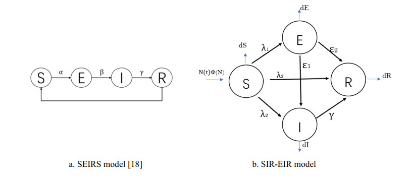
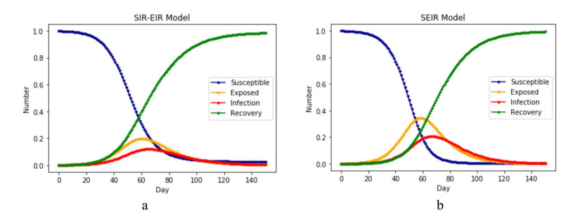
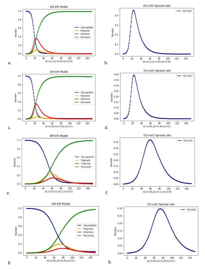
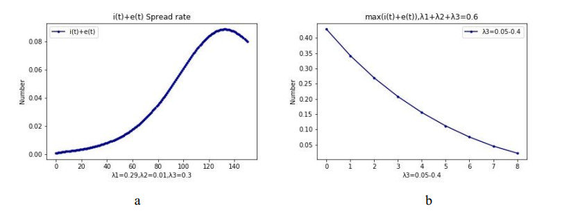
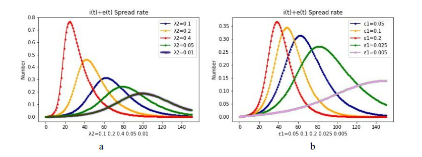
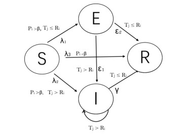
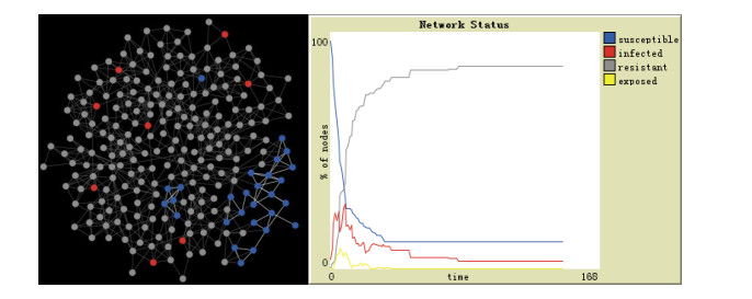
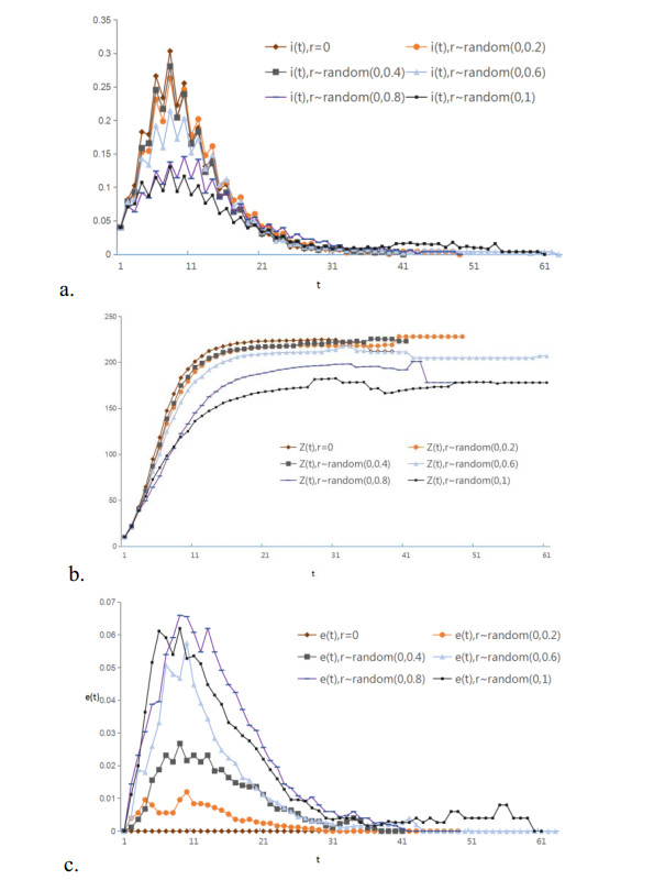
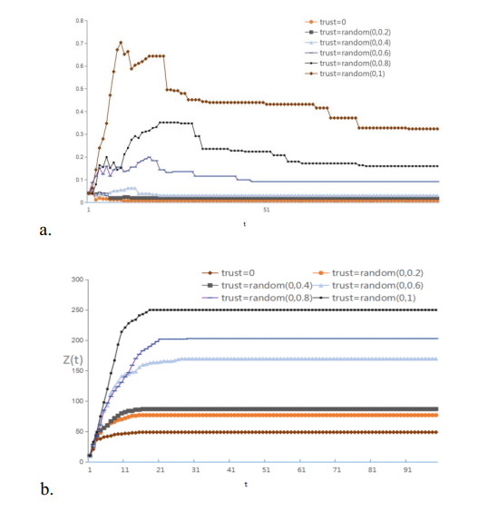
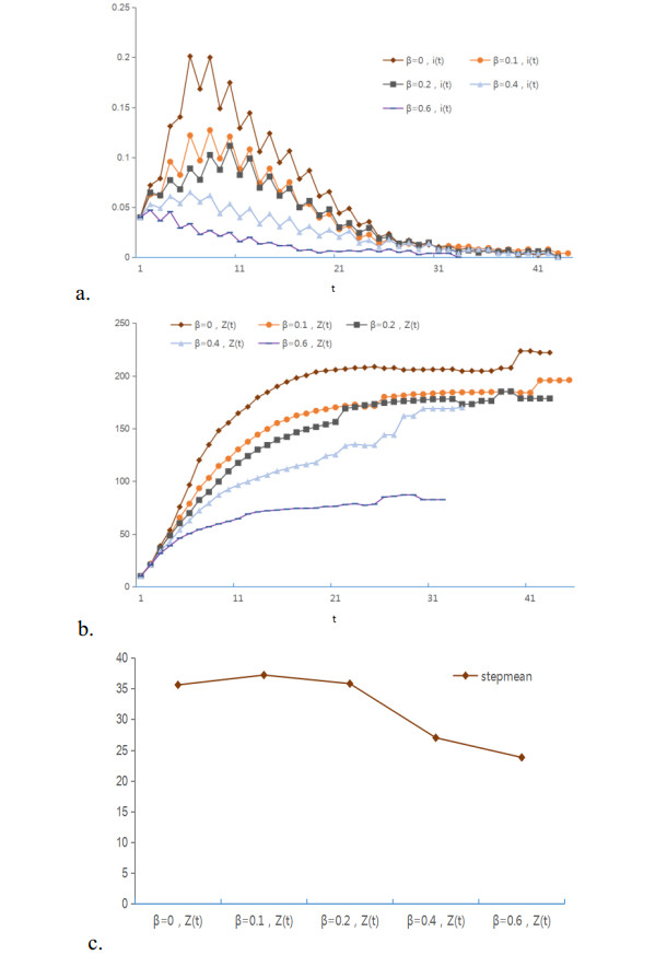
Meme transmission has become an important way of information dissemination. Three transfer paths were added to the classic infectious disease storehouse model in this study based on characteristics of meme transmission. Individual heterogeneity factors such as individual interest, risk perception and trust perception were used to construct a meme transmission model named Individual Heterogeneity SEIR (IHSEIR) model. Equilibrium of the model and the basic reproduction number were obtained using mean-field theory. Effects of individual heterogeneity factors on meme propagation were analyzed through Multi-Agent simulation. The findings showed that individual interest has a significant effect on the propagation range and speed of meme. A low-level overall trust of the system was correlated with higher risk perception among individuals, which is not conducive for the propagation of meme. Effect of regulation and intervention in the process of meme transmission was significantly lower compared with that at the initial state of transmission.
Citation: Jun Zhai, Bilin Xu. Research on meme transmission based on individual heterogeneity[J]. Mathematical Biosciences and Engineering, 2021, 18(5): 5176-5193. doi: 10.3934/mbe.2021263
Meme transmission has become an important way of information dissemination. Three transfer paths were added to the classic infectious disease storehouse model in this study based on characteristics of meme transmission. Individual heterogeneity factors such as individual interest, risk perception and trust perception were used to construct a meme transmission model named Individual Heterogeneity SEIR (IHSEIR) model. Equilibrium of the model and the basic reproduction number were obtained using mean-field theory. Effects of individual heterogeneity factors on meme propagation were analyzed through Multi-Agent simulation. The findings showed that individual interest has a significant effect on the propagation range and speed of meme. A low-level overall trust of the system was correlated with higher risk perception among individuals, which is not conducive for the propagation of meme. Effect of regulation and intervention in the process of meme transmission was significantly lower compared with that at the initial state of transmission.

| [1] | R. Dawkins, The Selfish Gene, Science Press, 1981. |
| [2] | S. Blackmore, The Meme Machine, Oxford University Press, 1999. |
| [3] | K. Distin, The Selfish Meme, Cambridge University Press, 2005. |
| [4] | D. Gruhl, R. Guha, D. Liben-Nowell, A. Tomkins, Information diffusion through blogspace, in Proceedings of the 13th International Conference on World Wide Web, 2004,491-501. |
| [5] | B. H. Spitzberg, Toward a model of meme diffusion(M3D), Commun. Theor., 24 (2014): 311-339. |
| [6] | C. Bauckhage, K. Kersting, F. Hadiji, Mathematical models of fads explain the temporal dynamics of internet memes, in Proceedings of the International AAAI Conference on Web and Social Media, (Vol. 7, No. 1), Cambridge, Massachusetts, USA, 2013. |
| [7] | C. Bauckhage, Insights into Internet Memes, in Proceedings of the International AAAI conference on Weblogs and Social Media, Barcelona, Catalonia, Spain, 2011 |
| [8] | C. Bauckhage, K. Kersting, Strong Regularities in Growth and Decline of Popularity of Social Media Services, arXiv preprint arXiv, (2014), 1406.6529. |
| [9] |
L. Wang, B. C. Wood, An epidemiological approach to model the viral propagation of memes, Appl. Math. Model., 35 (2011), 5442-5447. doi: 10.1016/j.apm.2011.04.035

|
| [10] | I. Miller, G. Cupchik, Meme creation and sharing processes: individuals shaping the masses, arXiv preprint arXiv, (2014), 14067579. |
| [11] |
X. Wei, N. C. Valler, B. A. Prakash, I. Neamtiu, M. Faloutsos, C. Faloutsos, Competing memes propagation on networks: A network science perspective, IEEE J. Sel. Areas Commun., 31 (2013), 1049-1060. doi: 10.1109/JSAC.2013.130607
|
| [12] | D. Freitag, E. Chow, P. Kalmar, T. Muezzinoglu, J. Niekrasz, A Corpus of Online Discussions for Research into Linguistic Memes, In Web as Corpus Workshop (WAC7), (2012), 14. |
| [13] | S. Towers, O. Patterson-Lomba, C. Castillo-Chavez, Emerging disease dynamics: The case of Ebola, SIAM News, 47 (2014), 2-3. |
| [14] | J. Kwiatkowska, J. Gutowska, Memetics on the facebook, Polish J. Manag. Stud., 5 (2012), 305-314. |
| [15] | A. Smailhodvic, K. Andrew, L. Hahn, P. C. Womble, C. Webb, Sample NLPDE and NLODE social-media modeling of information transmission for infectious diseases: Case Study Ebola, arXiv preprint arXiv, (2014), 1501.00198. |
| [16] | W. Sun, W. Yuan, H. Cui, P. Song, Simulation of Internet meme transmission process based on infectious disease model (in Chinese), Research in Communication Power, 26 (2019), 262-263. |
| [17] | D. Zhang, The Construction and Simulation of Internet Meme Model: A Case Study of 'Friendship Boat' (in Chinese), New Century Library, 3 (2017), 57-62. |
| [18] | R. Sachak-Patwa, N. T. Fadai, R. A. Van Gorder, Understanding viral video dynamics through an epidemic modelling approach, Physica A, 502 (2018), 416-435. |
| [19] | R. Sachak-Patwa, N. T. Fadai, R. A. Van Gorder, Modeling multi-group dynamics of related viral videos with delay differential equations, Physica A, 512 (2019), 197-217. |
| [20] | W. O. Kermack, A. G. McKendrick, A contribution to the mathematical theory of epidemics, Proc. R. Soc. A, Math. Phys. Eng. Sci., 115 (1927), 700-721. |
| [21] |
A. Korobeinikov, P. K. Maini, Nonlinear incidence and stability of infectious disease models, Math. Med. Biol., 22 (2005), 113-128. doi: 10.1093/imammb/dqi001
|
| [22] | H. Huang, M. Wang, The reaction-diffusion system for an SIR epidemic model with a free boundary, Discrete Contin. Dyn. Syst., 20 (2015), 2039-2050 |
| [23] |
G. Huang, Y. Takeuchi, W. Ma, D. Wei, Global stability for delay SIR and SEIR epidemic models with nonlinear incidencerate, Bull. Math. Biol., 72 (2010), 1192-1207 doi: 10.1007/s11538-009-9487-6
|
| [24] |
W. Ma, M. Song, Y. Takeuchi, Global stability of an SIR epidemic model with time delay, Appl. Math. Lett., 17 (2004), 1141-1145. doi: 10.1016/j.aml.2003.11.005
|
| [25] |
S. Han, C. Lei, Global Stability of Equilibria of a Diffusive SEIR Epidemic Model with Nonlinear Incidence, Appl. Math. Lett., 98 (2019), 114-120. doi: 10.1016/j.aml.2019.05.045
|
| [26] | E. Ávila-Vales, E. Rivero-Esquivel, G. E. García-Almeida, Global Dynamics of a Periodic SEIRS Model with General Incidence Rate, Int. J. Differ. Equ., 2017 (2017), 1-14. |
Figures(10) / Tables(2)

Jun Zhai, Bilin Xu. Research on meme transmission based on individual heterogeneity[J]. Mathematical Biosciences and Engineering, 2021, 18(5): 5176-5193. doi: 10.3934/mbe.2021263


 DownLoad: