Semi-supervised learning has always been a hot topic in machine learning. It uses a large number of unlabeled data to improve the performance of the model. This paper combines the co-training strategy and random forest to propose a novel semi-supervised regression algorithm: semi-supervised random forest regression model based on co-training and grouping with information entropy (E-CoGRF), and applies it to the evaluation of depression symptoms severity. The algorithm inherits the ensemble characteristics of random forest, and combines well with co-training. In order to balance the accuracy and diversity of co-training random forests, the algorithm proposes a grouping strategy to decision trees. Moreover, the information entropy is used to measure the confidence, which avoids unnecessary repeated training and improves the efficiency of the model. In the practical application of evaluation of depression symptoms severity, we collect cognitive behavioral data of emotional conflict based on the depressive affective disorder. And on this basis, feature construction and normalization preprocessing are carried out. Finally, the test is conducted on 35 labeled and 80 unlabeled depression patients. The result shows that the proposed algorithm obtains MAE (Mean Absolute Error) = 3.63 and RMSE (Root Mean Squared Error) = 4.50, which is better than other semi-supervised regression algorithms. The proposed method effectively solves the modeling difficulties caused by insufficient labeled samples, and has important reference value for the diagnosis of depression symptoms severity.
Citation: Shengfu Lu, Xin Shi, Mi Li, Jinan Jiao, Lei Feng, Gang Wang. Semi-supervised random forest regression model based on co-training and grouping with information entropy for evaluation of depression symptoms severity[J]. Mathematical Biosciences and Engineering, 2021, 18(4): 4586-4602. doi: 10.3934/mbe.2021233
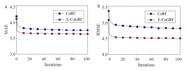
Semi-supervised learning has always been a hot topic in machine learning. It uses a large number of unlabeled data to improve the performance of the model. This paper combines the co-training strategy and random forest to propose a novel semi-supervised regression algorithm: semi-supervised random forest regression model based on co-training and grouping with information entropy (E-CoGRF), and applies it to the evaluation of depression symptoms severity. The algorithm inherits the ensemble characteristics of random forest, and combines well with co-training. In order to balance the accuracy and diversity of co-training random forests, the algorithm proposes a grouping strategy to decision trees. Moreover, the information entropy is used to measure the confidence, which avoids unnecessary repeated training and improves the efficiency of the model. In the practical application of evaluation of depression symptoms severity, we collect cognitive behavioral data of emotional conflict based on the depressive affective disorder. And on this basis, feature construction and normalization preprocessing are carried out. Finally, the test is conducted on 35 labeled and 80 unlabeled depression patients. The result shows that the proposed algorithm obtains MAE (Mean Absolute Error) = 3.63 and RMSE (Root Mean Squared Error) = 4.50, which is better than other semi-supervised regression algorithms. The proposed method effectively solves the modeling difficulties caused by insufficient labeled samples, and has important reference value for the diagnosis of depression symptoms severity.

| [1] | G Casalino, G Castellano, F Galetta, K. Kaczmarek-Majer, Dynamic incremental semi-supervised fuzzy clustering for bipolar disorder episode prediction, in International Conference on Discovery Science, Springer, Cham, (2020), 79-93. |
| [2] | J. C. Wakefield and S. Demazeux, Introduction: Depression, one and many, Sadness or Depression?, Netherlands, Springer, 2016, 1-15. |
| [3] | M. E. Gerbasi, A. Eldar-Lissai, S. Acaster, M. Fridman, V. Bonthapally, P. Hodgkins, et al., Associations between commonly used patient-reported outcome tools in postpartum depression clinical practice and the Hamilton Rating Scale for Depression, Arch. Women's Mental Health, 23 (2020), 727-735. |
| [4] | C. L. Allan, C. E. Sexton, N. Filippini, A. Topiwala, A. Mahmood, E. Zsoldos, et al., Sub-threshold depressive symptoms and brain structure: A magnetic resonance imaging study within the Whitehall Ⅱ cohort, J. Affective Disord., 204 (2016), 219-225. |
| [5] | X. Li, Z. Jing, B. Hu, J. Zhu, N. Zhong, M. Li, et al., A resting-state brain functional network study in MDD based on minimum spanning tree analysis and the hierarchical clustering, Complexity, 2017 (2017), 9514369. |
| [6] | K. Yoshida, Y. Shimizu, J. Yoshimoto, M. Takamura, G. Okada, Y. Okamoto, et al., Prediction of clinical depression scores and detection of changes in whole-brain using resting-state functional MRI data with partial least squares regression, Plos One, 12 (2017), e0179638. |
| [7] | S. Sun, X. Li, J. Zhu, Y. Wang, R. La, X. Zhang, et al., Graph theory analysis of functional connectivity in major depression disorder with high-density resting state EEG data, IEEE Trans. Neural Syst. Rehabil. Eng., 27 (2019), 429-439. |
| [8] |
U. R. Acharya, S. L. Oh, Y Hagiwara, J. Tan, H. Adeli, D. P. Subha, Automated EEG-based screening of depression using deep convolutional neural network, Comput. Methods Prog. Biomed., 161 (2018), 103-113. doi: 10.1016/j.cmpb.2018.04.012

|
| [9] |
R. W. Lam, S. H. Kennedy, R. S. McIntyre, A. Khullar, Cognitive dysfunction in major depressive disorder: effects on psychosocial functioning and implications for treatment, Can. J. Psychiatry, 59 (2014), 649-654. doi: 10.1177/070674371405901206
|
| [10] | R. S. McIntyre, D. S. Cha, J. K. Soczynska, H. O. Woldeyohannes, L. A. Gallaugher, P. Kudlow, et al., Cognitive deficits and functional outcomes in major depressive disorder: determinants, substrates, and treatment interventions, Depression Anxiety, 30 (2013), 515-527. |
| [11] | Y. Kang, X. Jiang, Y. Yin, Y. Shang, X. Zhou, Deep transformation learning for depression diagnosis from facial images, in Chinese Conference on Biometric Recognition, Springer, Cham, (2017), 13-22. |
| [12] | A. Haque, M. Guo, A. S. Miner, F. Li, Measuring depression symptom severity from spoken language and 3D facial expressions, preprint, arXiv: 1811.08592. |
| [13] | M. Muzammel, H. Salam, Y. Hoffmann, M. Chetouani, A. Othmani, AudVowelConsNet: A phoneme-level based deep CNN architecture for clinical depression diagnosis, Mach. Learn. Appl., 2 (2020), 100005. |
| [14] | J. Zhu, J. Li, X. Li, J. Rao, Y. Hao, Z. Ding, et al., Neural basis of the emotional conflict processing in major depression: ERPs and source localization analysis on the N450 and P300 components, Front. Human Neurosci., 12 (2018), 214. |
| [15] |
B. W. Haas, K. Omura, R. T. Constable, T. Canli, Interference produced by emotional conflict associated with anterior cingulate activation, Cognit. Affective Behav. Neurosci., 6 (2006), 152-156. doi: 10.3758/CABN.6.2.152
|
| [16] |
T. Armstrong, B. O. Olatunji, Eye tracking of attention in the affective disorders: a meta-analytic review and synthesis, Clin. Psychol. Rev., 32 (2012), 704-723. doi: 10.1016/j.cpr.2012.09.004
|
| [17] |
A. Duque, C. Vázquez, Double attention bias for positive and negative emotional faces in clinical depression: Evidence from an eye-tracking study, J Behav. Ther. Exp. Psychiatry, 46 (2015), 107-114. doi: 10.1016/j.jbtep.2014.09.005
|
| [18] |
S. P. Karparova, A. Kersting, T. Suslow, Disengagement of attention from facial emotion in unipolar depression, Psychiatry Clin. Neurosci., 59 (2005), 723-729. doi: 10.1111/j.1440-1819.2005.01443.x
|
| [19] |
M. P. Caligiuri, J. Ellwanger, Motor and cognitive aspects of motor retardation in depression, J. Affective Disord., 57 (2000), 83-93. doi: 10.1016/S0165-0327(99)00068-3
|
| [20] |
A. Etkin, T. Egner, D. M. Peraza, E. R. Kandel, J. Hirsch, Resolving emotional conflict: a role for the rostral anterior cingulate cortex in modulating activity in the amygdala, Neuron, 51 (2006), 871-882. doi: 10.1016/j.neuron.2006.07.029
|
| [21] | K Mohan, A Seal, O Krejcar, A. Yazidi, FER-net: facial expression recognition using deep neural net, Neural Comput. Appl., (2021), 1-12. |
| [22] | K Mohan, A Seal, O Krejcar, A. Yazidi, Facial expression recognition using local gravitational force descriptor-based deep convolution neural networks, IEEE Trans. Instrum. Meas., 70 (2020), 1-12. |
| [23] | Z. Zhou, M. Li, Semi-supervised regression with co-training, in IJCAI, (2005), 908-913. |
| [24] | M. A. Lei, W. Xili, Semi-supervised regression based on support vector machine co-training, Comput. Eng. Appl., 47 (2011), 177-180. |
| [25] | Y. Q. Li, M. Tian, A semi-supervised regression algorithm based on co-training with SVR-KNN, in Advanced Materials Research, Trans Tech Publications Ltd, (2014), 2914-2918. |
| [26] |
L. Bao, X. Yuan, Z. Ge, Co-training partial least squares model for semi-supervised soft sensor development, Chemom. Intell. Lab. Syst., 147 (2015), 75-85. doi: 10.1016/j.chemolab.2015.08.002
|
| [27] | D. Li, Y. Liu, D. Huang, Development of semi-supervised multiple-output soft-sensors with Co-training and tri-training MPLS and MRVM, Chemom. Intell. Lab. Syst., 199 (2020), 103970. |
| [28] | M. F. A. Hady, F. Schwenker and G. Palm, Semi-supervised learning for regression with co-training by committee, in International Conference on Artificial Neural Networks, Springer, Berlin, Heidelberg, (2009), 121-130. |
| [29] | F. Saitoh, Predictive modeling of corporate credit ratings using a semi-supervised random forest regression, 2016 IEEE International Conference on Industrial Engineering and Engineering Management (IEEM), IEEE, (2016), 429-433. |
| [30] |
J. Levatić, M. Ceci, D. Kocev, S. Džeroski, Self-training for multi-target regression with tree ensembles, Knowl. Based Syst., 123 (2017), 41-60. doi: 10.1016/j.knosys.2017.02.014
|
| [31] |
S. Xue, S. Wang, X. Kong, J. Qiu, Abnormal neural basis of emotional conflict control in treatment-resistant depression: An event-related potential study, Clin. EEG Neurosci., 48 (2017), 103-110. doi: 10.1177/1550059416631658
|
| [32] | N. Tottenham, J. W. Tanaka, A. C. Leon, T. McCarry, M. Nurse, T. A. Hare, et al., The NimStim set of facial expressions: Judgments from untrained research participants, Psychiatry Res., 168 (2009), 242-249. |
| [33] | M. Lei, J. Yang, S. Wang, L. Zhao, P. Xia, G. Jiang, et al., Semi-supervised modeling and compensation for the thermal error of precision feed axes, Int. J. Adv. Manuf. Technol., 104 (2019), 4629-4640. |
Figures(5) / Tables(7)

Shengfu Lu, Xin Shi, Mi Li, Jinan Jiao, Lei Feng, Gang Wang. Semi-supervised random forest regression model based on co-training and grouping with information entropy for evaluation of depression symptoms severity[J]. Mathematical Biosciences and Engineering, 2021, 18(4): 4586-4602. doi: 10.3934/mbe.2021233


 DownLoad: