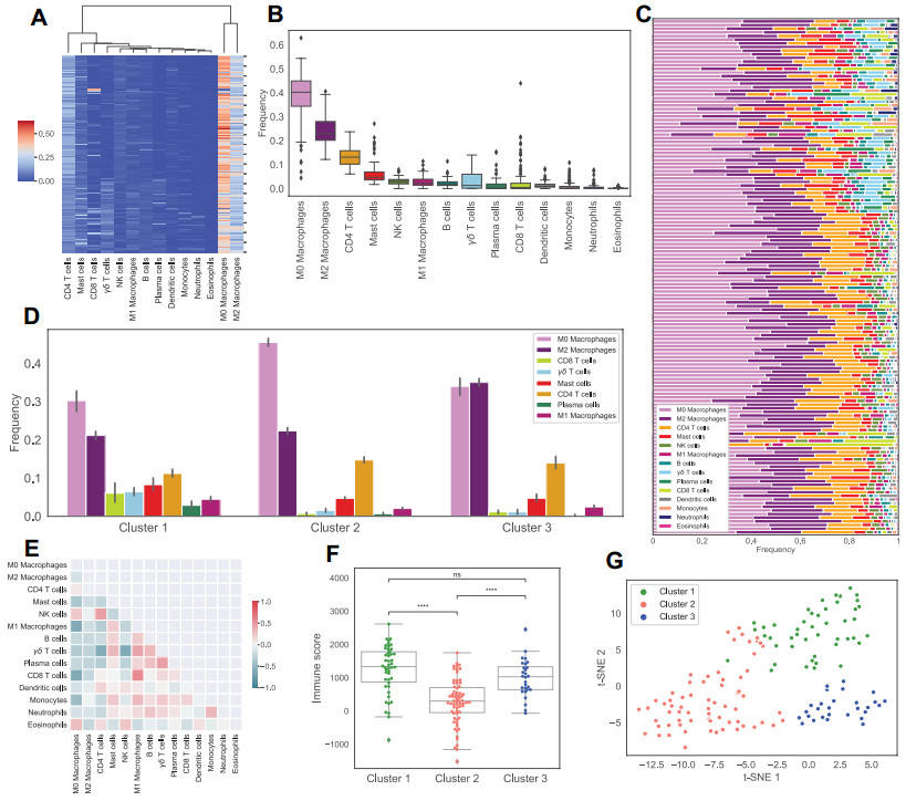
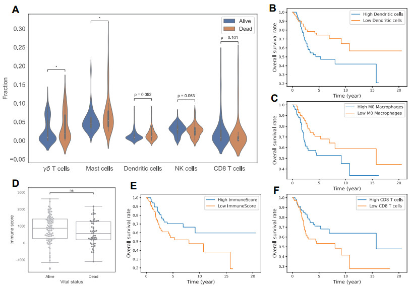
Tumor immune microenvironment has been shown to be important in predicting the tumor progression and the outcome of treatments. This work aims to identify different immune patterns in osteosarcoma and their clinical characteristics. We use the latest and best performing deconvolution method, CIBERSORTx, to obtain the relative abundance of 22 immune cells. Then we cluster patients based on their estimated immune abundance and study the characteristics of these clusters, along with the relationship between immune infiltration and outcome of patients. We find that abundance of CD8 T cells, NK cells and M1 Macrophages have a positive association with prognosis, while abundance of $ \gamma \delta $ T cells, Mast cells, M0 Macrophages and Dendritic cells have a negative association with prognosis. Accordingly, the cluster with the lowest proportion of CD8 T cells, M1 Macrophages and highest proportion of M0 Macrophages has the worst outcome among clusters. By grouping patients with similar immune patterns, we are also able to suggest treatments that are specific to the tumor microenvironment.
Citation: Trang Le, Sumeyye Su, Leili Shahriyari. Immune classification of osteosarcoma[J]. Mathematical Biosciences and Engineering, 2021, 18(2): 1879-1897. doi: 10.3934/mbe.2021098
Tumor immune microenvironment has been shown to be important in predicting the tumor progression and the outcome of treatments. This work aims to identify different immune patterns in osteosarcoma and their clinical characteristics. We use the latest and best performing deconvolution method, CIBERSORTx, to obtain the relative abundance of 22 immune cells. Then we cluster patients based on their estimated immune abundance and study the characteristics of these clusters, along with the relationship between immune infiltration and outcome of patients. We find that abundance of CD8 T cells, NK cells and M1 Macrophages have a positive association with prognosis, while abundance of $ \gamma \delta $ T cells, Mast cells, M0 Macrophages and Dendritic cells have a negative association with prognosis. Accordingly, the cluster with the lowest proportion of CD8 T cells, M1 Macrophages and highest proportion of M0 Macrophages has the worst outcome among clusters. By grouping patients with similar immune patterns, we are also able to suggest treatments that are specific to the tumor microenvironment.

| [1] |
M. Kansara, M. W. Teng, M. J. Smyth, D. M. Thomas, Translational biology of osteosarcoma, Nat. Rev. Cancer, 14 (2014), 722–735. doi: 10.1038/nrc3838

|
| [2] | American Cancer Society, What Cause Osteosarcoma?, 2021. Available from: https://www.cancer.org/cancer/osteosarcoma/causes-risks-prevention/what-causes.html. |
| [3] |
X. He, Z. Gao, H. Xu, Z. Zhang, P. Fu, A meta-analysis of randomized control trials of surgical methods with osteosarcoma outcomes, J. Orthop. Surg. Res., 12 (2017), 5. doi: 10.1186/s13018-016-0500-0
|
| [4] |
P. A. Meyers, C. L. Schwartz, M. D. Krailo, J. H. Healey, M. L. Bernstein, D. Betcher, et al., Osteosarcoma: the addition of muramyl tripeptide to chemotherapy improves overall survival-a report from the Children's Oncology Group, J. Clin. Oncol., 26 (2008), 633–638. doi: 10.1200/JCO.2008.14.0095
|
| [5] |
F. Conforti, L. Pala, V. Bagnardi, T. De Pas, M. Martinetti, G. Viale, et al., Cancer immunotherapy efficacy and patients' sex: a systematic review and meta-analysis, Lancet Oncol., 19 (2018), 737–746. doi: 10.1016/S1470-2045(18)30261-4
|
| [6] |
Y. T. Lee, Y. J. Tan, C. E. Oon, Molecular targeted therapy: treating cancer with specificity, Eur. J. Pharmacol., 834 (2018), 188–196. doi: 10.1016/j.ejphar.2018.07.034
|
| [7] |
K. L. Davis, E. Fox, M. S. Merchant, J. M. Reid, R. A. Kudgus, X. Liu, et al., Nivolumab in children and young adults with relapsed or refractory solid tumours or lymphoma (ADVL1412): A multicentre, open-label, single-arm, phase 1–2 trial, Lancet Oncol., 21 (2020), 541–550. doi: 10.1016/S1470-2045(20)30023-1
|
| [8] | S. I. Grivennikov, F. R. Greten, M. Karin, Immunity, inflammation, and cancer, Cell, 140 (2010), 883–899. |
| [9] |
T. Kitamura, B. Z. Qian, J. W. Pollard, Immune cell promotion of metastasis, Nat. Rev. Immunol., 15 (2015), 73–86. doi: 10.1038/nri3789
|
| [10] |
J. B. Swann, M. J. Smyth, Immune surveillance of tumors, J. Clin. Invest., 117 (2007), 1137–1146. doi: 10.1172/JCI31405
|
| [11] |
F. Pagès, A. Kirilovsky, B. Mlecnik, M. Asslaber, M. Tosolini, G. Bindea, et al., In Situ Cytotoxic and Memory T Cells Predict Outcome in Patients With Early-Stage Colorectal Cancer, J. Clin. Oncol., 27 (2009), 5944–5951. doi: 10.1200/JCO.2008.19.6147
|
| [12] |
J. Yao, W. Xi, Y. Zhu, H. Wang, X. Hu, J. Guo, Checkpoint molecule PD-1-assisted CD8+ T lymphocyte count in tumor microenvironment predicts overall survival of patients with metastatic renal cell carcinoma treated with tyrosine kinase inhibitors, Cancer Manag. Res., 10 (2018), 3419–3431. doi: 10.2147/CMAR.S172039
|
| [13] |
N. Tarek, D. A. Lee, Natural killer cells for osteosarcoma, Adv. Exp. Med. Biol., 804 (2014), 341–353. doi: 10.1007/978-3-319-04843-7_19
|
| [14] |
Z. Li, Potential of human $\gamma \delta$ T cells for immunotherapy of osteosarcoma, Mol. Biol. Rep., 40 (2013), 427–437. doi: 10.1007/s11033-012-2077-y
|
| [15] |
J. R. Heath, A. Ribas, P. S. Mischel, Single-cell analysis tools for drug discovery and development, Nat. Rev. Drug. Discov., 15 (2016), 204–216. doi: 10.1038/nrd.2015.16
|
| [16] | T. Le, R. A. Aronow, A. Kirshtein, L. Shahriyari, A review of digital cytometry methods: estimating the relative abundance of cell types in a bulk of cells, Brief. Bioinform., 2020 (2020), bbaa219. |
| [17] | S. Su, S. Akbarinejad, L. Shahriyari, Immune classification of clear cell renal cell carcinoma, 2020. Available from: https://www.biorxiv.org/content/10.1101/2020.07.03.187047v1.abstract. |
| [18] |
A. Kirshtein, S. Akbarinejad, W. Hao, T. Le, S. Su, R. A. Aronow, et al., Data driven mathematical model of colon cancer progression, J. Clin. Med., 9 (2020), 3947. doi: 10.3390/jcm9123947
|
| [19] |
L. Li, L. Shen, J. Ma, Q. Zhou, M. Li, H. Wu, et al., Evaluating distribution and prognostic value of new tumor-infiltrating lymphocytes in HCC based on a scRNA-seq study with CIBERSORTx, Front. Med., 7 (2020), 451. doi: 10.3389/fmed.2020.00451
|
| [20] |
L. Huang, H. Chen, Y. Xu, J. Chen, Z. Liu, Q. Xu, Correlation of tumor-infiltrating immune cells of melanoma with overall survival by immunogenomic analysis, Cancer Med., 9 (2020), 8444–8456. doi: 10.1002/cam4.3466
|
| [21] |
A. M. Newman, C. B. Steen, C. L. Liu, A. J. Gentles, A. A. Chaudhuri, F. Scherer, et al., Determining cell type abundance and expression from bulk tissues with digital cytometry, Nat. Biotechnol., 37 (2019), 773–782. doi: 10.1038/s41587-019-0114-2
|
| [22] |
C. Zhang, J. H. Zheng, Z. H. Lin, H. Y. Lv, Z. M. Ye, Y. P. Chen, et al., Profiles of immune cell infiltration and immune-related genes in the tumor microenvironment of osteosarcoma, Aging, 12 (2020), 3486–3501. doi: 10.18632/aging.102824
|
| [23] |
W. Hong, H. Yuan, Y. Gu, M. Liu, Y. Ji, Z. Huang, et al., Immune-related prognosis biomarkers associated with osteosarcoma microenvironment, Cancer Cell Int., 20 (2020), 1–12. doi: 10.1186/s12935-019-1086-5
|
| [24] |
Y. Yu, H. Zhang, T. Ren, Y. Huang, X. Liang, W. Wang, et al., Development of a prognostic gene signature based on an immunogenomic infiltration analysis of osteosarcoma, J. Cell. Mol. Med., 24 (2020), 11230–11242. doi: 10.1111/jcmm.15687
|
| [25] |
C. Hu, C. Liu, S. Tian, Y. Wang, R. Shen, H. Rao, et al., Comprehensive analysis of prognostic tumor microenvironment-related genes in osteosarcoma patients, BMC Cancer, 20 (2020), 1–11. doi: 10.1186/s12885-019-6169-0
|
| [26] | Y. Tang, Z. Gu, Y. Fu, J. Wang, CXCR3 from chemokine receptor family correlates with immune infiltration and predicts poor survival in osteosarcoma, Biosci. Rep., 39 (2019), 1–12. |
| [27] |
J. Niu, T. Yan, W. Guo, W. Wang, Z. Zhao, T. Ren, et al., Identification of Potential Therapeutic Targets and Immune Cell Infiltration Characteristics in Osteosarcoma Using Bioinformatics Strategy, Front. Oncol., 10 (2020), 1628. doi: 10.3389/fonc.2020.01628
|
| [28] | L. Q. Li, L. H. Zhang, Y. Zhang, X. C. Lu, Y. Zhang, Y. K. Liu, et al., Construction of immune-related gene pairs signature to predict the overall survival of osteosarcoma patients, Aging, 12 (2020), 22906–22926. |
| [29] |
T. Zhang, Y. Nie, H. Xia, Y. Zhang, K. Cai, X. Chen, et al., Identification of Immune-Related Prognostic Genes and LncRNAs Biomarkers Associated With Osteosarcoma Microenvironment, Front. Oncol., 10 (2020), 1109. doi: 10.3389/fonc.2020.01109
|
| [30] | W. Yuan, Y. Deng, E. Ren, G. Zhang, Z. Wu, Q. Xie, Analysis of Immune Infiltration Pattern in Osteosarcoma and Its Clinical Significance, Res. Sq., 2020 (2020), 1–26. |
| [31] |
Y. J. Song, Y. Xu, X. Zhu, J. Fu, C. Deng, H. Chen, et al., Immune Landscape of the Tumor Microenvironment Identifies Prognostic Gene Signature CD4/CD68/CSF1R in Osteosarcoma, Front. Oncol., 10 (2020), 1198. doi: 10.3389/fonc.2020.01198
|
| [32] | T. Chen, L. Zhao, Patrolling monocytes inhibit osteosarcoma metastasis to the lung, Aging, 12 (2020), 23004–23016. |
| [33] |
C. Deng, Y. Xu, J. Fu, X. Zhu, H. Chen, H. Xu, et al., Reprograming the tumor immunologic microenvironment using neoadjuvant chemotherapy in osteosarcoma, Cancer Sci., 111 (2020), 1899–1909. doi: 10.1111/cas.14398
|
| [34] |
X. Yang, W. Zhang, P. Xu, NK cell and macrophages confer prognosis and reflect immune status in osteosarcoma, J. Cell. Biochem., 120 (2019), 8792–8797. doi: 10.1002/jcb.28167
|
| [35] | C. C. Wu, H. C. Beird, J. A. Livingston, S. Advani, A. Mitra, S. Cao, et al., Immuno-genomic landscape of osteosarcoma, Nat. Commun., 11 (2020), 1–11. |
| [36] |
A. M. Newman, C. L. Liu, M. R. Green, A. J. Gentles, W. Feng, Y. Xu, et al., Robust enumeration of cell subsets from tissue expression profiles, Nat. Methods, 12 (2015), 453–457. doi: 10.1038/nmeth.3337
|
| [37] | K. Yoshihara, M. Shahmoradgoli, E. Martínez, R. Vegesna, H. Kim, W. Torres-Garcia, et al., Inferring tumour purity and stromal and immune cell admixture from expression data, Nat. Commun., 4 (2013), 1–11. |
| [38] | G. Qiao, H. Miao, Y. Yi, D. Wang, B. Liu, Y. Zhang, et al., Genetic association between CTLA-4 variations and osteosarcoma risk: Case-control study, Int. J. Clin. Exp. Med., 9 (2016), 9598–9602. |
| [39] | C. Zhang, W. H. Hou, X. X. Ding, X. Wang, H. Zhao, X. W. Han, et al., Association of cytotoxic T-lymphocyte antigen-4 polymorphisms with malignant bone tumors risk: A meta-analysis, Asian Pac. J. Cancer Prev., 17 (2016), 3783–3789. |
| [40] |
K. Schroder, P. J. Hertzog, T. Ravasi, D. A. Hume, Interferon-$\gamma$: an overview of signals, mechanisms and functions, J. Leukocyte Biol., 75 (2004), 163–189. doi: 10.1189/jlb.0603252
|
| [41] |
H. Wajant, The role of TNF in cancer, Results Probl. Cell Differ., 49 (2009), 1–15. doi: 10.1007/400_2008_26
|
| [42] | National Center for Biotechnology Information, IL1B interleukin 1 beta, 2021. Available from: https://www.ncbi.nlm.nih.gov/gene/3553. |
| [43] |
Y. S. Li, Q. Liu, H. B. He, W. Luo, The possible role of insulin-like growth factor-1 in osteosarcoma, Curr. Prob. Cancer, 43 (2019), 228–235. doi: 10.1016/j.currproblcancer.2018.08.008
|
| [44] | T. Jentzsch, B. Robl, M. Husmann, B. Bode-Lesniewska, B. Fuchs, Worse prognosis of osteosarcoma patients expressing IGF-1 on a tissue microarray, Anticancer Res., 34 (2014), 3881–3890. |
| [45] | J. W. Martin, M. Zielenska, G. S. Stein, A. J. van Wijnen, J. A. Squire, The role of RUNX2 in osteosarcoma oncogenesis, Sarcoma, 2011 (2011), 1–13. |
| [46] |
A. Roos, L. Satterfield, S. Zhao, D. Fuja, R. Shuck, M. J. Hicks, et al., Loss of Runx2 sensitises osteosarcoma to chemotherapy-induced apoptosis, Br. J. Cancer, 113 (2015), 1289–1297. doi: 10.1038/bjc.2015.305
|
| [47] | S. Miwa, T. Shirai, N. Yamamoto, K. Hayashi, A. Takeuchi, K. Igarashi, et al., Current and emerging targets in immunotherapy for osteosarcoma, J. Oncol., 2019 (2019), 1–8. |
| [48] | K. Wang, A. T. Vella, Regulatory T cells and cancer: a two-sided story. Immunol. Invest., 45 (2016), 797–812. |
| [49] | M. F. Heymann, D. Heymann, Immune environment and osteosarcoma, in Osteosarcoma-Biology, Behavior and Mechanisms, InTech: London, UK, (2017), 105–120. |
| [50] | T. T. Maciel, I. C. Moura, O. Hermine, The role of mast cells in cancers, F1000Prime Rep., 7 (2015), 5–10. |
| [51] | Y. Zhao, C. Niu, J. Cui, Gamma-delta ($\gamma\; \delta$) T Cells: friend or foe in cancer development?, J. Transl. Med., 16 (2018), 1–13. |
| [52] |
M. F. Heymann, F. Lézot, D. Heymann, The contribution of immune infiltrates and the local microenvironment in the pathogenesis of osteosarcoma, Cell. Immunol., 343 (2019), 103711. doi: 10.1016/j.cellimm.2017.10.011
|
| [53] |
A. Lamora, J. Talbot, M. Mullard, B. L. Royer, F. Redini, F. Verrecchia, TGF-$\beta$ signaling in bone remodeling and osteosarcoma progression, J. Clin. Med., 5 (2016), 96. doi: 10.3390/jcm5110096
|
| [54] |
I. Corre, F. Verrecchia, V. Crenn, F. Redini, V. Trichet, The osteosarcoma microenvironment: a complex but targetable ecosystem, Cells, 9 (2020), 1–25. doi: 10.3390/cells9020278
|
| [55] | D. S. Chen, I. Mellman, Oncology meets immunology: the cancer-immunity cycle. Immunity, 39 (2013), 1–10. |
| [56] | R. J. Motzer, B. Escudier, D. F. McDermott, S. George, H. J. Hammers, S. Srinivas, et al., Nivolumab versus Everolimus in Advanced Renal-Cell Carcinoma. New Engl. J. Med., 373 (2015), 1803–1813. |
| [57] |
J. Dine, R. Gordon, Y. Shames, M. Kasler, M. Barton-Burke, Immune checkpoint inhibitors: An innovation in immunotherapy for the treatment and management of patients with cancer, Asia Pac. J. Oncol. Nurs., 4 (2017), 127–135. doi: 10.4103/apjon.apjon_4_17
|
| [58] |
S. L. Topalian, F. S. Hodi, J. R. Brahmer, S. N. Gettinger, D. C. Smith, D. F. McDermott, et al., Safety, activity, and immune correlates of anti–PD-1 antibody in cancer, New Engl. J. Med., 366 (2012), 2443–2454. doi: 10.1056/NEJMoa1200690
|
| [59] |
S. Koyama, E. A. Akbay, Y. Y. Li, G. S. Herter-Sprie, K. A. Buczkowski, W. G. Richards, et al., Adaptive resistance to therapeutic PD-1 blockade is associated with upregulation of alternative immune checkpoints, Nat. Commun., 7 (2016), 10501. doi: 10.1038/ncomms10501
|
| [60] |
F. S. Hodi, S. J. O'Day, D. F. McDermott, R. W. Weber, J. A. Sosman, J. B. Haanen, et al., Improved survival with ipilimumab in patients with metastatic melanoma, New Engl. J. Med., 363 (2010), 711–723. doi: 10.1056/NEJMoa1003466
|
| [61] |
H. A. Tawbi, M. Burgess, V. Bolejack, B. A. Van Tine, S. M. Schuetze, J. Hu, et al., Pembrolizumab in advanced soft-tissue sarcoma and bone sarcoma (SARC028): a multicentre, two-cohort, single-arm, open-label, phase 2 trial, Lancet Oncol., 18 (2017), 1493–1501. doi: 10.1016/S1470-2045(17)30624-1
|
| [62] |
P. Thanindratarn, D. C. Dean, S. D. Nelson, F. J. Hornicek, Z. Duan, Advances in immune checkpoint inhibitors for bone sarcoma therapy, J. Bone Oncol., 15 (2019), 100221. doi: 10.1016/j.jbo.2019.100221
|
| [63] |
Ö. Sercan, G. J. Hämmerling, B. Arnold, T. Schüler, Cutting Edge: Innate Immune Cells Contribute to the IFN-$\gamma$-Dependent Regulation of Antigen-Specific CD8 + T Cell Homeostasis, J. Immunol., 176 (2006), 735–739. doi: 10.4049/jimmunol.176.2.735
|
| [64] |
B. D. X. Lascelles, W. S. Dernell, M. T. Correa, M. Lafferty, C. M. Devitt, C. A. Kuntz CA, et al., Improved survival associated with postoperative wound infection in dogs treated with limb-salvage surgery for osteosarcoma, Ann. Surg. Oncol., 12 (2005), 1073–1083. doi: 10.1245/ASO.2005.01.011
|
| [65] |
Y. Chen, S. F. Xu, M. Xu, X. C. Yu, Postoperative infection and survival in osteosarcoma patients: Reconsideration of immunotherapy for osteosarcoma, Mol. Clin. Oncol., 3 (2015), 495–500. doi: 10.3892/mco.2015.528
|
| [66] |
J. Karbach, A. Neumann, K. Brand, C. Wahle, E. Siegel, M. Maeurer, et al., Phase I clinical trial of mixed bacterial vaccine (Coley's toxins) in patients with NY-ESO-1 expressing cancers: Immunological effects and clinical activity, Clin. Cancer Res., 18 (2012), 5449–5459. doi: 10.1158/1078-0432.CCR-12-1116
|
| [67] | Z. Ling, G. Fan, D. Yao, J. Zhao, Y. Zhou, J. Feng, et al., MicroRNA-150 functions as a tumor suppressor and sensitizes osteosarcoma to doxorubicin-induced apoptosis by targeting RUNX2, Exp. Ther. Med., 19 (2019), 481–488. |
| [68] |
Z. Wang, Z. Wang, B. Li, S. Wang, T. Chen, Z. Ye, Innate immune cells: A potential and promising cell population for treating osteosarcoma, Front. Immunol., 10 (2019), 1–19. doi: 10.3389/fimmu.2019.00001
|
| [69] |
Q. Zhou, M. Xian, S. Xiang, D. Xiang, X. Shao, J. Wang, et al., All-trans retinoic acid prevents osteosarcoma metastasis by inhibiting M2 polarization of tumor-associated macrophages, Cancer Immunol. Res., 5 (2017), 547–559. doi: 10.1158/2326-6066.CIR-16-0259
|
| [70] |
Y. Kimura, M. Sumiyoshi, Resveratrol prevents tumor growth and metastasis by inhibiting lymphangiogenesis and M2 macrophage activation and differentiation in tumor-associated macrophages, Nutr. Cancer, 68 (2016), 667–678. doi: 10.1080/01635581.2016.1158295
|
| [71] |
Y. Kimura, M. Sumiyoshi, Antitumor and antimetastatic actions of dihydroxycoumarins (esculetin or fraxetin) through the inhibition of M2 macrophage differentiation in tumor-associated macrophages and/or G1 arrest in tumor cells, Eur. J. Pharmacol., 746 (2015), 115–125. doi: 10.1016/j.ejphar.2014.10.048
|
Figures(6)

Trang Le, Sumeyye Su, Leili Shahriyari. Immune classification of osteosarcoma[J]. Mathematical Biosciences and Engineering, 2021, 18(2): 1879-1897. doi: 10.3934/mbe.2021098


 DownLoad: