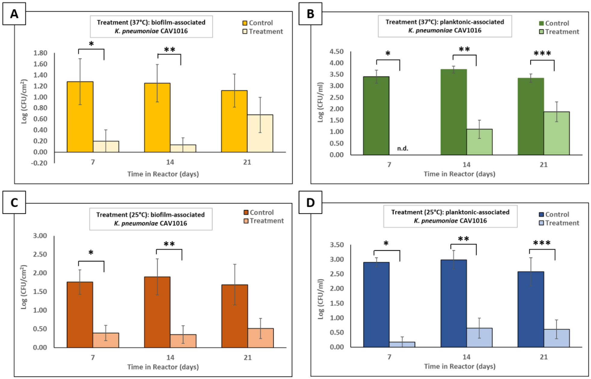
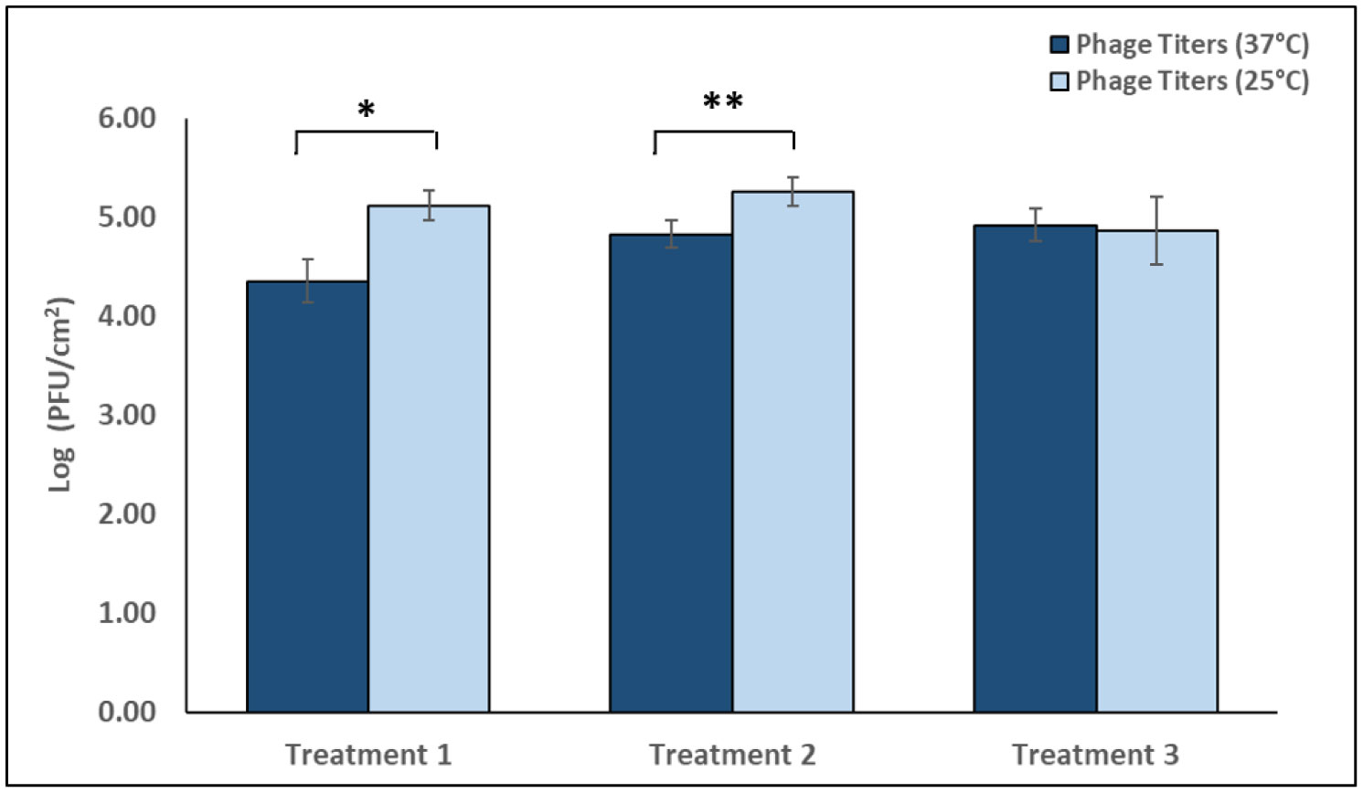
The p-traps of hospital handwashing sinks represent a potential reservoir for antimicrobial-resistant organisms of major public health concern, such as carbapenemase-producing KPC+ Klebsiella pneumoniae (CPKP). Bacteriophages have reemerged as potential biocontrol agents, particularly against biofilm-associated, drug-resistant microorganisms. The primary objective of our study was to formulate a phage cocktail capable of targeting a CPKP strain (CAV1016) at different stages of colonization within polymicrobial drinking water biofilms using a CDC biofilm reactor (CBR) p-trap model. A cocktail of four CAV1016 phages, all exhibiting depolymerase activity, were isolated from untreated wastewater using standard methods. Biofilms containing Pseudomonas aeruginosa, Micrococcus luteus, Stenotrophomonas maltophilia, Elizabethkingia anophelis, Cupriavidus metallidurans, and Methylobacterium fujisawaense were established in the CBR p-trap model for a period of 28 d. Subsequently, CAV1016 was inoculated into the p-trap model and monitored over a period of 21 d. Biofilms were treated for 2 h at either 25 °C or 37 °C with the phage cocktail (109 PFU/ml) at 7, 14, and 21 d post-inoculation. The effect of phage treatment on the viability of biofilm-associated CAV1016 was determined by plate count on m-Endo LES agar. Biofilm heterotrophic plate counts (HPC) were determined using R2A agar. Phage titers were determined by plaque assay. Phage treatment reduced biofilm-associated CAV1016 viability by 1 log10 CFU/cm2 (p < 0.05) at 7 and 14 d (37 °C) and 1.4 log10 and 1.6 log10 CFU/cm2 (p < 0.05) at 7 and 14 d, respectively (25 °C). No significant reduction was observed at 21 d post-inoculation. Phage treatment had no significant effect on the biofilm HPCs (p > 0.05) at any time point or temperature. Supplementation with a non-ionic surfactant appears to enhance phage association within biofilms. The results of this study suggest the potential of phages to control CPKP and other carbapenemase-producing organisms associated with microbial biofilms in the healthcare environment.
Citation: Ariel J. Santiago, Maria L. Burgos-Garay, Leila Kartforosh, Mustafa Mazher, Rodney M. Donlan. Bacteriophage treatment of carbapenemase-producing Klebsiella pneumoniae in a multispecies biofilm: a potential biocontrol strategy for healthcare facilities[J]. AIMS Microbiology, 2020, 6(1): 43-63. doi: 10.3934/microbiol.2020003
The p-traps of hospital handwashing sinks represent a potential reservoir for antimicrobial-resistant organisms of major public health concern, such as carbapenemase-producing KPC+ Klebsiella pneumoniae (CPKP). Bacteriophages have reemerged as potential biocontrol agents, particularly against biofilm-associated, drug-resistant microorganisms. The primary objective of our study was to formulate a phage cocktail capable of targeting a CPKP strain (CAV1016) at different stages of colonization within polymicrobial drinking water biofilms using a CDC biofilm reactor (CBR) p-trap model. A cocktail of four CAV1016 phages, all exhibiting depolymerase activity, were isolated from untreated wastewater using standard methods. Biofilms containing Pseudomonas aeruginosa, Micrococcus luteus, Stenotrophomonas maltophilia, Elizabethkingia anophelis, Cupriavidus metallidurans, and Methylobacterium fujisawaense were established in the CBR p-trap model for a period of 28 d. Subsequently, CAV1016 was inoculated into the p-trap model and monitored over a period of 21 d. Biofilms were treated for 2 h at either 25 °C or 37 °C with the phage cocktail (109 PFU/ml) at 7, 14, and 21 d post-inoculation. The effect of phage treatment on the viability of biofilm-associated CAV1016 was determined by plate count on m-Endo LES agar. Biofilm heterotrophic plate counts (HPC) were determined using R2A agar. Phage titers were determined by plaque assay. Phage treatment reduced biofilm-associated CAV1016 viability by 1 log10 CFU/cm2 (p < 0.05) at 7 and 14 d (37 °C) and 1.4 log10 and 1.6 log10 CFU/cm2 (p < 0.05) at 7 and 14 d, respectively (25 °C). No significant reduction was observed at 21 d post-inoculation. Phage treatment had no significant effect on the biofilm HPCs (p > 0.05) at any time point or temperature. Supplementation with a non-ionic surfactant appears to enhance phage association within biofilms. The results of this study suggest the potential of phages to control CPKP and other carbapenemase-producing organisms associated with microbial biofilms in the healthcare environment.

| [1] |
Leitner E, Zarfel G, Luxner J, et al. (2015) Contaminated handwashing sinks as the source of a clonal outbreak of KPC-2-producing Klebsiella oxytoca on a hematology ward. Antimicrob Agents Ch 59: 714-716. doi: 10.1128/AAC.04306-14

|
| [2] |
Regev-Yochay G, Smollan G, Tal I, et al. (2018) Sink traps as the source of transmission of OXA-48–producing Serratia marcescens in an intensive care unit. Infect Control Hosp Epidemiol 39: 1307-1315. doi: 10.1017/ice.2018.235
|
| [3] |
Donlan RM (2002) Biofilms: microbial life on surfaces. Emerging infect dis 8: 881-890. doi: 10.3201/eid0809.020063
|
| [4] |
Tofteland S, Naseer U, Lislevand JH, et al. (2013) A long-term low-frequency hospital outbreak of KPC-producing Klebsiella pneumoniae involving intergenus plasmid diffusion and a persisting environmental reservoir. PLoS One 8: e59015. doi: 10.1371/journal.pone.0059015
|
| [5] |
Lowe C, Willey B, O'Shaughnessy A, et al. (2012) Outbreak of extended-spectrum β-lactamase-producing Klebsiella oxytoca infections associated with contaminated handwashing sinks (1). Emerging Infect Dis 18: 1242-1247. doi: 10.3201/eid1808.111268
|
| [6] |
Carling PC (2018) Wastewater drains: epidemiology and interventions in 23 carbapenem-resistant organism outbreaks. Infect Control Hosp Epidemiol 39: 972-979. doi: 10.1017/ice.2018.138
|
| [7] |
Vergara-López S, Domínguez MC, Conejo MC, et al. (2013) Wastewater drainage system as an occult reservoir in a protracted clonal outbreak due to metallo-β-lactamase-producing Klebsiella oxytoca. Clin Microbiol Infect 19: E490-E498. doi: 10.1111/1469-0691.12288
|
| [8] |
Stone PW (2009) Economic burden of healthcare-associated infections: an American perspective. Expert Rev Pharmacoeconomics Outcomes Res 9: 417-422. doi: 10.1586/erp.09.53
|
| [9] |
Al-Tawfiq JA, Tambyah PA (2014) Healthcare associated infections (HAI) perspectives. J Infect Public Health 7: 339-344. doi: 10.1016/j.jiph.2014.04.003
|
| [10] |
Logan LK, Weinstein RA (2017) The epidemiology of carbapenem-resistant enterobacteriaceae: the impact and evolution of a global menace. J Infect Dis 215: S28-S36. doi: 10.1093/infdis/jiw282
|
| [11] |
Gupta N, Limbago BM, Patel JB, et al. (2011) Carbapenem-resistant enterobacteriaceae: epidemiology and prevention. Clin Infect Dis 53: 60-67. doi: 10.1093/cid/cir202
|
| [12] | Jacob J, Klein E, Laxminarayan R, et al. (2013) Vital signs: carbapenem-resistant enterobacteriaceae. MMWR Morbid Mortal We 62: 165-170. |
| [13] |
Kizny Gordon AE, Mathers AJ, Cheong EYL, et al. (2017) The hospital water environment as a reservoir for carbapenem-resistant organisms causing hospital-acquired infections—a systematic review of the literature. Clinl Infect Dis 64: 1435-1444. doi: 10.1093/cid/cix132
|
| [14] |
De Geyter D, Blommaert L, Verbraeken N, et al. (2017) The sink as a potential source of transmission of carbapenemase-producing Enterobacteriaceae in the intensive care unit. Antimicrob resist infect control 6: 24-24. doi: 10.1186/s13756-017-0182-3
|
| [15] |
Roux D, Aubier B, Cochard H, et al. (2013) Contaminated sinks in intensive care units: an underestimated source of extended-spectrum beta-lactamase-producing Enterobacteriaceae in the patient environment. J Hosp Infect 85: 106-111. doi: 10.1016/j.jhin.2013.07.006
|
| [16] |
Abedon ST (2017) Active bacteriophage biocontrol and therapy on sub-millimeter scales towards removal of unwanted bacteria from foods and microbiomes. AIMS Microbiol 3: 649-688. doi: 10.3934/microbiol.2017.3.649
|
| [17] |
Ramirez K, Cazarez-Montoya C, Lopez-Moreno HS, et al. (2018) Bacteriophage cocktail for biocontrol of Escherichia coli O157:H7: Stability and potential allergenicity study. PLoS One 13: e0195023. doi: 10.1371/journal.pone.0195023
|
| [18] |
Lehman SM, Donlan RM (2015) Bacteriophage-mediated control of a two-species biofilm formed by microorganisms causing catheter-associated urinary tract infections in an in vitro urinary catheter model. Antimicrob Agents Ch 59: 1127-1137. doi: 10.1128/AAC.03786-14
|
| [19] |
Hughes KA, Sutherland IW, Jones MV (1998) Biofilm susceptibility to bacteriophage attack: the role of phage-borne polysaccharide depolymerase. Microbiology 144: 3039-3047. doi: 10.1099/00221287-144-11-3039
|
| [20] |
Azeredo J, Sutherland IW (2008) The use of phages for the removal of infectious biofilms. Curr Pharm Biotechnol 9: 261-266. doi: 10.2174/138920108785161604
|
| [21] |
Majkowska-Skrobek G, Latka A, Berisio R, et al. (2018) Phage-borne depolymerases decrease Klebsiella pneumoniae resistance to innate defense mechanisms. Front Microbiol 9: 2517. doi: 10.3389/fmicb.2018.02517
|
| [22] |
Fish R, Kutter E, Wheat G, et al. (2016) Bacteriophage treatment of intransigent diabetic toe ulcers: a case series. J Wound Care 25: S27-S33. doi: 10.12968/jowc.2016.25.Sup7.S27
|
| [23] |
Mendes JJ, Leandro C, Corte-Real S, et al. (2013) Wound healing potential of topical bacteriophage therapy on diabetic cutaneous wounds. Wound Repair Regen 21: 595-603. doi: 10.1111/wrr.12056
|
| [24] | Carson L, Gorman SP, Gilmore BF (2010) The use of lytic bacteriophages in the prevention and eradication of biofilms of Proteus mirabilis and Escherichia coli. Pathog Dis 59: 447-455. |
| [25] |
Lungren MP, Donlan RM, Kankotia R, et al. (2014) Bacteriophage K antimicrobial-lock technique for treatment of Staphylococcus aureus central venous catheter–related infection: a leporine model efficacy analysis. J Vasc Interv Radiol 25: 1627-1632. doi: 10.1016/j.jvir.2014.06.009
|
| [26] |
Mathers AJ, Cox HL, Bonatti H, et al. (2009) Fatal cross infection by carbapenem-resistant Klebsiella in two liver transplant recipients. Transpl Infect Dis 11: 257-265. doi: 10.1111/j.1399-3062.2009.00374.x
|
| [27] |
Pierce VM, Simner PJ, Lonsway DR, et al. (2017) Modified carbapenem inactivation method for phenotypic detection of carbapenemase production among enterobacteriaceae. J Clin Microbiol 55: 2321. doi: 10.1128/JCM.00193-17
|
| [28] | Adams MH (1959) Bacteriophages London, United Kingdom: Interscience Publishers. |
| [29] | O'Toole GA (2011) Microtiter dish biofilm formation assay. J Vis Exp pii: 2437. |
| [30] | Donlan RM, Elliot DL, Kapp NJ, et al. (2000) Surfanctants for reducing bacterial adhesion onto surfaces. U.S., Patent, 6039965. editors. |
| [31] | Mazher M, Santiago A, Donlan R (2018) Control of Carbapenem-Resistant Klebsiella pneumoniae biofilms using a nonionic surfactant. |
| [32] |
Donlan RM, Piede JA, Heyes CD, et al. (2004) Model system for growing and quantifying Streptococcus pneumoniae biofilms in situ and in real time. Appl Environ Microbiol 70: 4980-4988. doi: 10.1128/AEM.70.8.4980-4988.2004
|
| [33] |
Goeres DM, Loetterle LR, Hamilton MA, et al. (2005) Statistical assessment of a laboratory method for growing biofilms. Microbiology 151: 757-762. doi: 10.1099/mic.0.27709-0
|
| [34] |
Armbruster CS, Forster TM, Donlan R, et al. (2012) A biofilm model developed to investigate survival and disinfection of Mycobacterium mucogenicum in potable water. Biofouling 28: 1129-1139. doi: 10.1080/08927014.2012.735231
|
| [35] |
Kotay S, Chai W, Guilford W, et al. (2017) Spread from the sink to the patient: in situ study using green fluorescent protein (GFP)-expressing Escherichia coli to model bacterial dispersion from hand-washing sink-trap reservoirs. Appl Environ Microbiol 83: e03327-03316. doi: 10.1128/AEM.03327-16
|
| [36] |
Kotsanas D, Wijesooriya WRPLI, Korman TM, et al. (2013) ‘Down the drain’: carbapenem-resistant bacteria in intensive care unit patients and handwashing sinks. Med J Aust 198: 267-269. doi: 10.5694/mja12.11757
|
| [37] | Kotay SM, Donlan RM, Ganim C, et al. (2019) Droplet-rather than aerosol-mediated dispersion is the primary mechanism of bacterial transmission from contaminated hand-washing sink traps. Appl Environ Microbiol 85: e01997-01918. |
| [38] |
Chan BK, Abedon ST (2015) Bacteriophages and their enzymes in biofilm control. Curr Pharm Design 21: 85-99. doi: 10.2174/1381612820666140905112311
|
| [39] |
Cornelissen A, Ceyssens P-J, T'Syen J, et al. (2011) The T7-related Pseudomonas putida phage φ15 displays virion-associated biofilm degradation properties. PLoS OneE 6: e18597. doi: 10.1371/journal.pone.0018597
|
| [40] |
Bodratti AM, Alexandridis P (2018) Formulation of poloxamers for drug delivery. J Funct Biomater 9: 11. doi: 10.3390/jfb9010011
|
| [41] |
Pitto-Barry A, Barry NPE (2014) Pluronic® block-copolymers in medicine: from chemical and biological versatility to rationalisation and clinical advances. Polym Chem 5: 3291-3297. doi: 10.1039/C4PY00039K
|
| [42] |
Percival SL, Mayer D, Malone M, et al. (2017) Surfactants and their role in wound cleansing and biofilm management. J Wound Care 26: 680-690. doi: 10.12968/jowc.2017.26.11.680
|
| [43] |
Das Ghatak P, Mathew-Steiner SS, Pandey P, et al. (2018) A surfactant polymer dressing potentiates antimicrobial efficacy in biofilm disruption. Sci Rep 8: 873-873. doi: 10.1038/s41598-018-19175-7
|
| [44] |
Seo Y, Bishop PL (2007) Influence of nonionic surfactant on attached biofilm formation and phenanthrene bioavailability during simulated surfactant enhanced bioremediation. Environ Sci Technol 41: 7107-7113. doi: 10.1021/es0701154
|
| [45] |
Simmons M, Drescher K, Nadell CD, et al. (2018) Phage mobility is a core determinant of phage-bacteria coexistence in biofilms. ISME J 12: 531-543. doi: 10.1038/ismej.2017.190
|
| [46] |
Tait K, Skillman LC, Sutherland IW (2002) The efficacy of bacteriophage as a method of biofilm eradication. Biofouling 18: 305-311. doi: 10.1080/0892701021000034418
|
| [47] |
Baghal Asghari F, Nikaeen M, Mirhendi H (2013) Rapid monitoring of Pseudomonas aeruginosa in hospital water systems: a key priority in prevention of nosocomial infection. FEMS Microbiol Lett 343: 77-81. doi: 10.1111/1574-6968.12132
|
| [48] | Cieplak T, Soffer N, Sulakvelidze A, et al. (2018) A bacteriophage cocktail targeting Escherichia coli reduces E. coli in simulated gut conditions, while preserving a non-targeted representative commensal normal microbiota. Gut Microbes 9: 391-399. |
| [49] |
Doolittle MM, Cooney JJ, Caldwell DE (1996) Tracing the interaction of bacteriophage with bacterial biofilms using fluorescent and chromogenic probes. J Ind Microbiol 16: 331-341. doi: 10.1007/BF01570111
|
| [50] |
Alexandridis P, Alan Hatton T (1995) Poly (ethylene oxide) poly (propylene oxide) poly (ethylene oxide) block copolymer surfactants in aqueous solutions and at interfaces: thermodynamics, structure, dynamics, and modeling. Colloids Surf A 96: 1-46. doi: 10.1016/0927-7757(94)03028-X
|
| [51] |
Choi YC, Morgenroth E (2003) Monitoring biofilm detachment under dynamic changes in shear stress using laser-based particle size analysis and mass fractionation. Water Sci Technol 47: 69-76. doi: 10.2166/wst.2003.0284
|
| [52] |
Roy B, Ackermann HW, Pandian S, et al. (1993) Biological inactivation of adhering Listeria monocytogenes by listeriaphages and a quaternary ammonium compound. Appl Environ Microbiol 59: 2914-2917. doi: 10.1128/AEM.59.9.2914-2917.1993
|
| [53] |
Sillankorva S, Neubauer P, Azeredo J (2010) Phage control of dual species biofilms of Pseudomonas fluorescens and Staphylococcus lentus. Biofouling 26: 567-575. doi: 10.1080/08927014.2010.494251
|
| [54] |
Chhibber S, Bansal S, Kaur S (2015) Disrupting the mixed-species biofilm of Klebsiella pneumoniae B5055 and Pseudomonas aeruginosa PAO using bacteriophages alone or in combination with xylitol. Microbiology 161: 1369-1377. doi: 10.1099/mic.0.000104
|
| [55] | Lenski RE (1988) Dynamics of Interactions between Bacteria and Virulent Bacteriophage. Advances in microbial ecology Boston, MA: Springer US, 1-44. |
| [56] |
Donlan RM (2009) Preventing biofilms of clinically relevant organisms using bacteriophage. Trends Microbiol 17: 66-72. doi: 10.1016/j.tim.2008.11.002
|
| [57] |
Meaden S, Koskella B (2013) Exploring the risks of phage application in the environment. Front Microbiol 4: 358-358. doi: 10.3389/fmicb.2013.00358
|
| [58] |
Colomer-Lluch M, Jofre J, Muniesa M (2011) Antibiotic resistance genes in the bacteriophage DNA fraction of environmental samples. PLoS One 6: e17549. doi: 10.1371/journal.pone.0017549
|
| [59] |
Nilsson AS (2019) Pharmacological limitations of phage therapy. Upsala J Med Sci 124: 218-227. doi: 10.1080/03009734.2019.1688433
|
| [60] |
Wang H, Edwards MA, Falkinham JO, et al. (2013) Probiotic approach to pathogen control in premise plumbing systems? a review. Environ Sci Technol 47: 10117-10128. doi: 10.1021/es402455r
|
| [61] |
Camper AK, LeChevallier MW, Broadaway SC, et al. (1985) Growth and persistence of pathogens on granular activated carbon filters. Appl Environ Microbiol 50: 1378. doi: 10.1128/AEM.50.6.1378-1382.1985
|
| [62] | Hu YOO, Hugerth LW, Bengtsson C, et al. (2018) Bacteriophages synergize with the gut microbial community to combat Salmonella. mSystems 3: e00119-00118. |
| [63] |
Zimlichman E, Henderson D, Tamir O, et al. (2013) Health care–associated Infections: a meta-analysis of costs and financial impact on the US Health Care System. JAMA Int Med 173: 2039-2046. doi: 10.1001/jamainternmed.2013.9763
|
| [64] |
Kim BR, Anderson JE, Mueller SA, et al. (2002) Literature review—efficacy of various disinfectants against Legionella in water systems. Water Res 36: 4433-4444. doi: 10.1016/S0043-1354(02)00188-4
|

Figures(7)

Ariel J. Santiago, Maria L. Burgos-Garay, Leila Kartforosh, Mustafa Mazher, Rodney M. Donlan. Bacteriophage treatment of carbapenemase-producing Klebsiella pneumoniae in a multispecies biofilm: a potential biocontrol strategy for healthcare facilities[J]. AIMS Microbiology, 2020, 6(1): 43-63. doi: 10.3934/microbiol.2020003


 DownLoad: