
Citation: Ahsan Javed, Awais Ahmad, Ali Tahir, Umair Shabbir, Muhammad Nouman, Adeela Hameed. Potato peel waste-its nutraceutical, industrial and biotechnological applacations[J]. AIMS Agriculture and Food, 2019, 4(3): 807-823. doi: 10.3934/agrfood.2019.3.807
[1] | Ye Sun, Daniel B. Work . Error bounds for Kalman filters on traffic networks. Networks and Heterogeneous Media, 2018, 13(2): 261-295. doi: 10.3934/nhm.2018012 |
[2] | Caterina Balzotti, Maya Briani, Benedetto Piccoli . Emissions minimization on road networks via Generic Second Order Models. Networks and Heterogeneous Media, 2023, 18(2): 694-722. doi: 10.3934/nhm.2023030 |
[3] | Matthieu Canaud, Lyudmila Mihaylova, Jacques Sau, Nour-Eddin El Faouzi . Probability hypothesis density filtering for real-time traffic state estimation and prediction. Networks and Heterogeneous Media, 2013, 8(3): 825-842. doi: 10.3934/nhm.2013.8.825 |
[4] | Maya Briani, Emiliano Cristiani . An easy-to-use algorithm for simulating traffic flow on networks: Theoretical study. Networks and Heterogeneous Media, 2014, 9(3): 519-552. doi: 10.3934/nhm.2014.9.519 |
[5] | Emiliano Cristiani, Smita Sahu . On the micro-to-macro limit for first-order traffic flow models on networks. Networks and Heterogeneous Media, 2016, 11(3): 395-413. doi: 10.3934/nhm.2016002 |
[6] | Samitha Samaranayake, Axel Parmentier, Ethan Xuan, Alexandre Bayen . A mathematical framework for delay analysis in single source networks. Networks and Heterogeneous Media, 2017, 12(1): 113-145. doi: 10.3934/nhm.2017005 |
[7] | Mauro Garavello, Benedetto Piccoli . On fluido-dynamic models for urban traffic. Networks and Heterogeneous Media, 2009, 4(1): 107-126. doi: 10.3934/nhm.2009.4.107 |
[8] | Dirk Helbing, Jan Siegmeier, Stefan Lämmer . Self-organized network flows. Networks and Heterogeneous Media, 2007, 2(2): 193-210. doi: 10.3934/nhm.2007.2.193 |
[9] | Fabio Della Rossa, Carlo D’Angelo, Alfio Quarteroni . A distributed model of traffic flows on extended regions. Networks and Heterogeneous Media, 2010, 5(3): 525-544. doi: 10.3934/nhm.2010.5.525 |
[10] | Tibye Saumtally, Jean-Patrick Lebacque, Habib Haj-Salem . A dynamical two-dimensional traffic model in an anisotropic network. Networks and Heterogeneous Media, 2013, 8(3): 663-684. doi: 10.3934/nhm.2013.8.663 |
Plant virus diseases are transmitted between plant individuals through vectors, including the tomato leaf roll virus and cassava mosaic virus. Plant viruses seriously affect crop yields, which can result in great economic losses and increased poverty, especially in developing countries [1]. According to [2], the annual wheat rust can cause yield loss of up to 80 percent, posing a great threat to global wheat production. Moreover, it is estimated that 12.5 million hectares were disturbed annually from 2003 to 2012 by plant disease, mostly Asia and Europe [3]. Therefore, the control of plant virus transmission remains a major economic and agricultural issue. The effective methods to control plant viruses include gene control, chemical control, and biological control. It is extremely effective to improve the antiviral ability of plants by changing genes, but it cannot be greatly used due to the high cost. Chemical control aims to control the vector by spraying insecticide. However, long-term use will not only pollute the environment, but also lead to drug resistance and increase the incidence of plant viruses. Biological control is widely used to control the spread of diseases by manually removing infected plants or introducing vector natural enemies, having significant effects and causing no pollution to the environment. Thus, biological control is increasingly used as an efficient method to control plant viruses.
Although biological control of plant viruses provides an effective method for controlling the spread of plant viruses, a successful control plan needs to understand the transmission mechanism of plant viruses in plants and vectors as well as the interaction between biological controllers and plants and vectors. Mathematical modeling has exerted a main and probably greater role in the epidemiology of plant viruses. Mathematical models enable us to comprehend the observed transmission routes and disease control of plant viruses, as well as grasp a deeper understanding of the mechanism of plant disease transmission dynamics. At present, there are numerous research achievements on biological control of plant viruses. As mentioned in [4], the authors consider the evolution of within-plant virus titer as the response to the application of various disease control methods. Moreover, they demonstrate that the process of new and improved disease control methods for viral diseases of vegetatively propagated staple food crops need to consider the evolutionary responses of the virus. According to [5], the authors concentrate on the contribution made by developing mathematical models with a scope of techniques that is extensive and their use for investigating plant virus disease epidemics. Their focus is on the extent to which models can help answer biological questions and raised questions in association with the epidemiology and ecology of plant viruses and the caused diseases. Based on [6,7], the authors applied optimization theory to investigate the plant vector virus model with continuous replanting and roguing, aiming to maximize the harvest of healthy plants and examine the best strategy to fight plant virus disease. In [8], the authors concentrate on a plant disease model with a latent period and nonautonomous phenomenon. Their focus is to explore the long-run behavior of the epidemic model.
In reality, considering that people control plant viruses at discrete time points, the establishment of impulse differential equations to reveal the propagation dynamics and control strategies of plant viruses has been favored by numerous scholars in recent years. In [9], the authors proposed and analyzed a plant virus disease model under periodic environment and pulse roguing. Based on their research, with the high infection rate, it can probably not be possible to eliminate the disease by easily roguing the infectious plant, and elevating the replanting rate is not conducive to the control of disease. In [10], to detect and design suitable plant disease control strategies, the authors proposed and investigated the dynamics of plant disease models by adopting continuous and impulsive cultural control strategies. Under a certain parameter space, it can be demonstrated that a nontrivial periodic solution occurs through a supercritical bifurcation. In [11], the authors formulated an epidemiological model for mosaic diseases considering plant and vector populations. They discovered that roguing is the most cost effective and beneficial management for mosaic disease eradication of plants if used at an appropriate rate and interval. In [12,13], with the purpose of eradicating plant diseases or keeping the number of infected plants below the economic threshold, the authors proposed and analyzed the plant disease models, including nonlinear impulsive functions and cultural control strategies. In [14], based on the purpose of minimizing losses and maximizing returns, the authors introduce a discontinuous plant disease model, which incorporates a threshold policy control. Their results suggest that we can adopt the proper replanting and roguing rates for designing the threshold policy, and thus the number of infected plants is within an acceptable level. Recently, pulse control methods can be applied in almost every field of applied science. The theoretical research and application analysis of pulse control can be found in many studies [15,16,17,18].
However, most of the above studies consider only (1) Continuous removal of infected plants or replanting of healthy plants, without considering removal of infected plants at discrete time points. (2) Pulse removes the infected plants without destroying the vector on the plants. Therefore, considering the shortcomings of the above literature, based on the above two points, we aim to develop a plant virus disease transmission model with nonlinear continuous and pulse control, analyze its dynamic behavior, and discuss the impact on plant virus disease control when removing infected plants and vectors on plants.
According to the model proposed in [19], we develop a vector-borne plant virus disease model with roguing control. The basic idea is that removing the infected plants will also eliminate the vectors on the plants. For plant populations, we classified plants into healthy plants X(t), infected plants Y(t), and the total number of plant populations at time t with N(t)=X(t)+Y(t). The recruitment rate of plant population is constant r. The newly recruited plants enter healthy plant populations X(t). The plant harvesting or death rate is denoted as g. Healthy plants are infected through contact with infection vectors, and the infection rate is k1V(t)N(t), where k1 is the probability of transmission from infected vectors to healthy plant. The expression of infection rate k1V(t)N(t) is acquired as follows. The probability that a vector selects a particular plant is assumed to be 1N(t), which is the probability of each plant selected by total N(t). Therefore, a plant receives in average M(t)N(t) contacts per unit of time. Later, the infection rate per healthy plant is offered by M(t)N(t)k1V(t)M(t). Considering using removal control on infected plants, the removal rate of diseased plants is α.
Vector populations are divided into non-infective U(t) and infective vectors V(t), and the total number of vector populations at time t denote M(t)=U(t)+V(t). The recruitment rate of vector population is constant μ. The newly recruited vectors enter non-infective vector populations U(t). The vector death rate is c. Uninfected vectors become infected through contact with infected plants, and the infection rate is k2Y(t)N(t), where k2 is the probability of transmission from infected plants to non-infective vectors.
The elimination of vectors occurs when the infected plants are removed with elimination rate of ραY(t)N(t) which is explained as follows. The average number of vector on each plant is M(t)N(t), and parameter ρ represents the elimination ratio of vectors on infected plants while removing each infected plant. Since the number of infected plants removed is αY(t), with the removal of the infected plants, the total number of eliminated vector is ραY(t)M(t)N(t). Thus, the elimination rate of vectors is ραY(t)M(t)N(t)1M(t). Therefore, our basic plant disease model reads as
{dX(t)dt=r−k1X(t)V(t)N(t)−gX(t),dY(t)dt=k1X(t)V(t)N(t)−gY(t)−αY(t),dU(t)dt=μ−k2U(t)Y(t)N(t)−cU(t)−ραU(t)Y(t)N(t),dV(t)dt=k2U(t)Y(t)N(t)−cV(t)−ραV(t)Y(t)N(t). | (2.1) |
We suppose that all parameter values are strictly positive.
Next, we indicate the boundedness of system (2.1), and it can follow from system (2.1) that:
dN(t)dt=r−gX(t)−(α+g)Y(t)≤r−gN(t), |
which suggests:
N(t)≤N(0)exp(−gt)+rg(1−exp(−gt))→rg,fort→∞. |
Similarly, we have
dM(t)dt=μ−cM(t)−ραM(t)Y(t)N(t)≤μ−cM(t), |
and thus, we obtain:
M(t)≤M(0)exp(−ct)+μc(1−exp(−ct))→μc,fort→∞. |
Therefore, the total plant population N(t) and vector population M(t) remain uniformly bounded. Moreover, the region
Ω={(X(t),Y(t),U(t),V(t))∈R4+:X(t)+Y(t)≤rg;U(t)+V(t)≤μc} | (2.2) |
is positively-invariant, indicating that this study concentrates on the dynamics of system (2.1) on the set Ω in the following.
With no disease in both of the populations(i.e., Y(t)=0, V(t)=0), the model (2.1) has one disease-free equilibrium E0=(N0,0,M0,0)=(rg,0,μc,0). By [20], we define the basic reproductive number
R0=√k1k2μgc2r(g+α). | (2.3) |
We note that
R0=√R01R02, |
where
R01=k1c |
refers to the expected number of plants that one vector infects via its infectious life time. R01 can be provided by the product of the infection rate of infectious vectors k1 and the average duration in the infectious stage 1c.
Similarly, we have
R02=k2M0N01(g+α)=k2gμcr(g+α), |
which is the expected number of vectors that one plant infects via its infectious life time. R02 is given by the product of the infection rate of infectious plants k2M0N0 and the average duration in the infectious stage 1g+α.
The basic reproduction number equals to the geometric mean of R01 and R02 since infection from plant to plant goes via one generation of vectors. In addition, the local asymptotic stability result of equilibrium E0 is provided:
Theorem 2.1. When R0<1, the disease-free equilibrium E0=(rg,0,μc,0) remains locally asymptotically stable in Ω.
Proof. The Jacobian matrix of system (2.1) at disease-free equilibrium E0 can be provided by:
JE0=(−g00−k10−(g+α)0k10−(k2+ρα)μgcr−c00k2μgcr0−c). |
The characteristic polynomial of JE0 can be expressed by:
P(λ)=(λ+g)(λ+c)φ(λ), |
where φ(λ)=λ2+a1λ+a2, with a1=c(g+α) and a2=c(g+α)(1−R20).
The roots of P(λ) are λ1=−g, λ2=−c and the others roots are the roots of φ(λ). Because R0<1, all coefficients of φ(λ) are always positive. Now, we just have to verify that the Routh-Hurwitz criterion holds for polynomial φ(λ). Therefore, setting H1=a1, H2=|a110a2|=a1a2. We have H1>0 and H2>0 if R0<1. Thus, by the Routh-Hurwitz criterion the trivial equilibrium E0 is locally asymptotically stable when R0<1.
In general, the biological implication of Theorem 2.1 is that with the basic reproduction number R0 being less than 1, a small number of infected vectors are introduced into the plant population, which will not cause disease outbreak, and the disease disappears in time. Nevertheless, in the following subsection, we present that the disease can persist even with R0<1.
With the purpose of determining whether there is an endemic equilibrium, we need to find the solution of the algebraic system of equations acquired through equating the right sides of system (2.1) to zero.
r−k1X∗(t)V∗(t)N∗(t)−gX∗(t)=0,k1X∗(t)V∗(t)N∗(t)−gY∗(t)−αY∗(t)=0,μ−k2U∗(t)Y∗(t)N∗(t)−cU∗(t)−ραU∗(t)Y∗(t)N∗(t)=0,k2U∗(t)Y∗(t)N∗(t)−cV∗(t)−ραV∗(t)Y∗(t)N∗(t)=0. | (2.4) |
For the sake of easier readability, we express the quantities as follows,
λ∗p=V∗N∗,λ∗v=Y∗N∗. |
By addressing the equations in the system (2.4) in terms of λ∗p and λ∗v, we can obtain:
X∗=rk1∗λ∗p+g,Y∗=rk1λ∗p(g+α)(k1λ∗p+g), | (2.5) |
and
U∗=μc+(k2+ρα)λ∗v,V∗=k2μλ∗v(c+ραλ∗v)((k2+ρα)λ∗v+c). | (2.6) |
By substituting (2.5) and (2.6) into the expression of λ∗p and λ∗v, we have
A(λ∗p)2+Bλ∗p+C=0, | (2.7) |
where
A=k21r(c+ρα)(c+ρα+k2)>0,B=k1(g+α)2c2rg(R2ρ−R20),C=c2r(g+α)2(1−R20),Rρ=√(2(c+ρα)+k2)r2c(g+α). |
We aimed to investigate the existence of endemic equilibria in the following cases:
(1) There is a unique endemic equilibrium if
(C<0) or (B<0 and C=0) or (B<0 and C>0 and B2−4AC=0);
(2) There are two endemic equilibria if
B<0 and C>0 and B2−4AC>0;
(3) There are no endemic equilibria otherwise.
Hence, we present the result in the theorem below.
Theorem 2.2. For system (2.1),
(1) If R0>1, there is a unique endemic equilibrium E∗.
(2) If R0=1 and B<0 there is a unique endemic equilibrium E∗. Otherwise, there exists no endemic equilibrium.
(3) If R0<1, and
(a) B<0 and B2−4AC>0, there are two equilibria E1 and E2.
(b) B<0 and B2−4AC=0, there exists a unique endemic equilibrium.
(c) There are no endemic equilibria otherwise.
Obviously, case (3) (item(a)) of Theorem 2.2 indicates the possibility of backward bifurcation in the model (2.1). Next, by applying the method of literature [21] to model (2.1), we present a rigorous proof that model (2.1) experiences a backward bifurcation.
Theorem 2.3. If cαg>r+k2+2ρα, the direction of the bifurcation of system (2.1) at R0=1 is backward.
Proof. Let k1 be the bifurcation parameter. To apply the method in reference[21], we introduce the notation x1=X, x2=Y, x3=U, x4=V, the system (2.1) becomes
{dx1dt=r−k1x1x4x1+x2−gx1:=f1(x1,x2,x3,x4),dx2dt=k1x1x4x1+x2−gx2−αx2:=f2(x1,x2,x3,x4),dx3dt=μ−k2x2x3x1+x2−cx3−ραx2x3x1+x2:=f3(x1,x2,x3,x4),dx4dt=k2x2x3x1+x2−cx4−ραx2x4x1+x2:=f4(x1,x2,x3,x4), | (2.8) |
with R0=1 corresponding to k1=k∗1=c2r(g+α)k2μg. The disease-free equilibrium is E0=(rg,0,μc,0). The linearization matrix of system (2.8) around the disease-free equilibrium when k1=k∗1 is
DE0f=(−g00−k∗10−(g+α)0k∗10−(k2+ρα)μgcr−c00k2μgcr0−c), |
where f=(f1,f2,f3,f4)′. Clearly, 0 indicates a simple eigenvalue of DE0f. A right eigenvector related to 0 eigenvalue is ω=[−cr(g+α)k2μg2,crk2μg,−k2+ραck2,1c]′, and the left eigenvector υ meeting ω⋅υ=1 is υ=[0,k2μgr(c+g+α),0,c(g+α)(c+g+α)]. Algebraic calculations demonstrate that
∂2f2∂x2∂x4=∂2f2∂x4∂x2=−cr(g+α)k2μ,∂2f4∂x2∂x1=∂2f4∂x1∂x2=−k2μg2cr2,∂2f4∂x22=−2k2μg2cr2,∂2f4∂x3∂x2=∂2f4∂x2∂x3=k2gr,∂2f4∂x4∂x2=∂2f4∂x2∂x4=−ραgr,∂2f2∂x2∂k1=1. |
The remaining of the second derivatives appear in the formula for a and b are all zero. The a and b presented in Theorem 4.1 of [21] are
a=n∑k,i,j=1υkωiωj∂2f∂xi∂xj(0,0),b=n∑k,i=1υkωi∂2f∂xi∂ϕ(0,0). |
Hence,
a=2c(g+α)k2μ(c+g+α)(cαg−(r+k2+2ρα)),b=k2μgcr(c+g+α)>0. |
By [21], if cαg>r+k2+2ρα, then a>0, and the direction of the bifurcation of system (2.1) at R0=1 is backward.
The backward bifurcation phenomenon indicates that with the basic reproductive number R0<1, the disease-free equilibrium is locally stable. Therefore, it is insufficient to only reduce the basic reproductive number R0<1 in order to eliminate the disease. Figure 1 depicts the associated bifurcation diagram. This clearly demonstrates the coexistence of two locally-asymptotically stable equilibria with R0<1, proving that the model (2.1) reveals the phenomenon of backward bifurcation. Therefore, to eradicate plant diseases, it is of necessity to increase α, and thus R0 is less than R0(α0), where R0(α0) is the threshold for the appearance of two endemic equilibria.
Figure 2 presents the occurrence of the backward bifurcation. In this study, R0<1, while according to the initial condition, the solution of the model (2.1) can approach either the endemic equilibrium point or the disease-free equilibrium point.
The current section extends model (2.1) by replacing the continuous infected plants with a periodic pulse roguing control strategy, which is shown to be more realistic. Therefore, our impulsive control model of plant virus diseases reads as
{dX(t)dt=r−k1X(t)V(t)N(t)−gX(t),dY(t)dt=k1X(t)V(t)N(t)−gY(t),dU(t)dt=μ−k2U(t)Y(t)N(t)−cU(t),dV(t)dt=k2U(t)Y(t)N(t)−cV(t),}t≠nT,X(t+)=(1−p)X(nT),Y(t+)=(1−α)Y(nT),U(t+)=(1−ραY(nT)N(nT)−ρpX(nT)N(nT))U(nT),V(t+)=(1−ραY(nT)N(nT))V(nT),}t=nT,X(0+)=X0,Y(0+)=Y0,U(0+)=U0,V(0+)=V0, | (3.1) |
where T indicates a fixed positive constant and suggests the periodic of the impulsive effect, where n∈N represents the positive integer set. The parameter α suggests the proportion of the infected plants, which is rogued at each pulse perturbation. Considering the inevitable impact of control measures on healthy plants, we use p representing the proportion of the healthy plants, which is rogued at each pulse perturbation. Here, we assume that p<α. Similar to the continuous model, the ratio of removing uninfected and infected vectors while removing plants is ραY(nT)N(nT). As there are only uninfected vectors on healthy plants, only uninfected vectors can be eliminated while removing healthy plants. The elimination ratio is ρpX(nT)N(nT), where ρ represents the vectors elimination rate of vectors, which probably means that some of the uninfected vectors and infected vectors will be occasionally eliminated due to the rogued plants.
When Y(t)=0, V(t)=0, then model (3.1) is the subsystem below:
{dX(t)dt=r−gX(t),dU(t)dt=μ−cU(t),}t≠nT,X(nT+)=(1−p)X(nT),U(nT+)=(1−ρp)U(nT),}t=nT,X(0+)=X0,U(0+)=U0, | (3.2) |
which presents the dynamics of the system in the absence of the infected plants and vectors. For system (3.2), we can address it in any impulsive interval (nT,(n+1)T] and obtain:
{X(t)=(X(nT+)−rg)exp(−g(t−nT))+rg,U(t)=(U(nT+)−μc)exp(−c(t−nT))+μc. | (3.3) |
Denote Xn=X(nT+) and Un=U(nT+), then:
{Xn+1=(1−p)Xnexp(−gT)+r(1−p)g(1−exp(−gT)),Un+1=(1−pρ)Xnexp(−cT)+μ(1−pρ)c(1−exp(−cT)). | (3.4) |
There is a steady state (X∗,U∗), which suggests that system (3.2) has a positive periodic solution (X∗(t),U∗(t)), where X∗(t)=(X∗−rg)exp(−g(t−nT))+rg, U∗(t)=(U∗−μc)exp(−c(t−nT))+μc with X∗=r(1−p)(1−exp(−gT))g(1−(1−p)exp(−gT)) and U∗=μ(1−pρ)(1−exp(−cT))c(1−(1−pρ)exp(−cT)). Hence, the following lemma can be obtained.
Lemma 3.1. System (3.2) has a positive periodic solution (X∗(t),U∗(t)). For any solution of (3.2), this study obtains X(t)→X∗(t), U(t)→U∗(t) as t→∞.
Proof. From (3.3) and (3.4), we obtain the solution of (3.2) as
{X(t)=(X0(1−p)nexp(−ngT)+(1−(1−p)nexp(−ngT))r(1−p)(1−exp(−gT))g(1−(1−p)exp(−gT))−rg)exp(−g(t−nT))+rg,U(t)=(U0(1−pρ)nexp(−ncT)+(1−(1−p)nexp(−ncT))μ(1−pρ)(1−exp(−ncT))c(1−(1−pρ)exp(−cT))−μc)exp(−c(t−nT))+μc, | (3.5) |
which indicates that X(t)→X∗(t) and U(t)→U∗(t) as n→∞ and t∈(nT,(n+1)T].
Therefore, system (3.1) has a disease-free periodic solution (X∗(t),0,U∗(t),0) and its stability has been solved.
To determine the stability of disease-free periodic solution (X∗(t),0,U∗(t),0) of system (3.1), we first calculate the basic reproduction number for the impulsive model (3.1) with the application of the next infection operator for the piecewise continuous periodic system being proposed in [22]. A(t) can be denoted as a n×n matrix, ΦA(.)(t) is suggested as the fundamental solution matrix of the linear ordinary differential system χ′=A(t)χ, and r(ΦA(.)(t)) is indicated as the spectral radius of ΦA(.)(t). Define X(t)=x(t)+X∗(t), Y(t)=y(t), U(t)=u(t)+U∗(t), V(t)=v(t), χ(t)=(x(t),u(t),y(t),v(t)). The corresponding linear system (3.1) reads as
{χ′(t)=G(t)χ(t),t≠nT,χ(t+)=Hχ(t),t=nT, | (3.6) |
where
G(t)=(G1(t)G2(t)OF(t)−Vr(t)),H=(H1H2OH3) | (3.7) |
with
G1(t)=(−g00−c),G2(t)=(0−k1−k2U∗(t)X∗(t)0),F(t)=(0k1k2U∗(t)X∗(t)0),Vr=(g00c) | (3.8) |
and
H1=(1−p001−ρp),H2=(00U∗(nT)ρ(p−α)X∗(nT)0),H3=(1−α001). | (3.9) |
Let ΦG(t)=Φij, 1≤i,j≤2, the fundamental solution matrix of system (3.6). Then, we have Φ′G(t)=G(t)ΦG(t) with the initial value ΦG(0)=I4. Based on the further computation, it is suggested that:
ΦG(t)=(exp(G1t)Φ12OΦF−Vr(t)), | (3.10) |
then we have
HΦG(T)=(H1exp(G1T)H2Φ12OH3ΦF−Vr(T)). | (3.11) |
It is obvious that r(H1exp(G1T))<1, by [22], the basic reproduction number for system (3.6) is provided as follow
R1=r(H3ΦF−Vr(T)). | (3.12) |
Using Floquet theory, if R1<1, we obtain the following result.
Theorem 3.2. The disease-free periodic solution (X∗(t),0,U∗(t),0) of model (3.1) is locally asymptotically stable when R1<1.
According to the persistence of the system, it can be found that plants (susceptible and infected) and vectors (susceptible and infected) can coexist, indicating that some conditions are satisfied, and the disease will not disappear. If we aim to eliminate the disease, the persistence indicates that control strategies are inefficient. Moreover, the permanent condition acquired from the exploration of the system can offer scientific support for determining the key factors causing failure and the effectiveness of control strategies, which later benefit us in establishing a good control program.
Theorem 3.3. When R2=r(H′3ΦF−Vr(T))>1, the disease is uniform persistence, i.e., there exists η>0 such that limt→∞infY(t)≥η>0,limt→∞infV(t)≥η>0. Here,
H′3=(1−α001−ρα). | (3.13) |
Proof. At first, we claim that there exists η>0, and thus:
limt→∞supY(t)≥η>0,limt→∞supV(t)≥η>0. | (3.14) |
Next, there is a t1>0 such that Y(t)<η,V(t)<η for all t≥t1. According to the first and third equations in system (3.1), the following can be obtained:
{dX(t)dt≥r−k1X(t)N(t)η−gX(t),t≠nT,dU(t)dt≥μ−k2U(t)N(t)η−cU(t),t≠nT,X(t+)=(1−p)X(t),t=nT,U(t+)≥(1−ρ(α+p))U(t),t=nT, | (3.15) |
and focus on the auxiliary system
{dz1(t)dt=r−k1η−gz1(t),t≠nT,dz2(t)dt=μ−k2z2(t)N(t)η−cz2(t),t≠nT,z1(t+)=(1−p)z1(t),t=nT,z2(t+)=(1−ρ(α+p))z2(t),t=nT. | (3.16) |
Since system (3.16) refers to a quasimonotone increasing system, based on the comparison theorem [23], the following can be obtained:
X(t)≥z1(t),U(t)≥z2(t). | (3.17) |
Using the solution of system (3.2), we acquire that model (3.16) admits a globally asymptotically stable positive periodic solution z∗(t)=(z∗1(t),z∗2(t)), and limη→0z∗(t)=(X∗(t),U∗(t)). Then, there exists η1 small enough and ε1>0 such that z∗1(t)≥X∗(t)−ε1 and z∗2(t)≥U∗(t)−ε1for η<η1. Therefore, by the comparison theorem, there is t2≥t1 and ε2>0, and thus
X(t)≥z1(t)≥z∗1(t)−ε2≥X∗(t)−ε1−ε2,U(t)≥z2(t)≥z∗2(t)−ε2≥U∗(t)−ε1−ε2. | (3.18) |
By substituting the above inequalities into the second and fourth equations of system (3.1), we acquire:
{dY(t)dt≥k1V(t)N(t)(X∗(t)−ε1−ε2)−gY(t),t≠nT,dV(t)dt≥k2Y(t)N(t)(U∗(t)−ε1−ε2)−cV(t),t≠nT,Y(t+)=(1−α)Y(t),t=nT,V(t+)=(1−ραY(t)N(t))V(t),t=nT. | (3.19) |
Supplementing the equations of plant population and vector population respectively provides:
{dN(t)dt=r−gN(t),t≠nT,dM(t)dt=μ−cM(t),t≠nT,N(t+)=(1−p)X(t)+(1−α)Y(t)≤(1−p)N(t),t=nT,M(t+)=(1−ρpX(t)N(t)−ραY(t)N(t))U(t)+(1−ραY(t)N(t))V(t)≤M(t),t=nT. | (3.20) |
Denoting (N1(t),M1(t)) is the solution of system (3.20) and (X1(t),U1(t)) as that of system (3.2). Comparing the equations in system (3.20) and (3.2) yields N1(t)≤X1(t),M1(t)≤U1(t). Since X1(t)≤X∗(t), U1(t)≤U∗(t), then we have N1(t)≤X∗(t), M1(t)≤U∗(t), and system (3.19) can be modified as
{dY(t)dt≥k1V(t)−gY(t),t≠nT,dV(t)dt≥k2U∗(t)X∗(t)Y(t)−cV(t),t≠nT,Y(t+)=(1−α)Y(t),t=nT,V(t+)=(1−ραY(t)N(t))V(t)≥(1−ρα)V(t),t=nT. | (3.21) |
Further, we concentrate on an auxiliary system
{dz3(t)dt=k1z4(t)−gz3(t),t≠nT,dz4(t)dt=k2U∗(t)X∗(t)z3(t)−cz4(t),t≠nT,z3(t+)=(1−α)z3(t),t=nT,z4(t+)=(1−ρα)z4(t),t=nT. | (3.22) |
It can be re-expressed as
{(dz3(t)dtdz4(t)dt)=(F(t)−Vr(t))(z3(t)z4(t)),t≠nT,(z3(t+)z4(t+))=H′3(z3(t)z4(t)),t=nT. | (3.23) |
The solution of system (3.23) can be shown as (z3(t),z4(t))T=ΦF−Vr(t−nT)(z3(nT+),z4(nT+))T. Then, (z3((n+1)T+),z4((n+1)T+))T=H′3ΦF−Vr(T)(z3(nT+),z4(nT+))T. While R2>1, z3(t)→∞ and z4(t)→∞ as t→∞. Consequently, limt→∞Y(t)=∞ and limt→∞V(t)=∞. Moreover, this is a contradiction with the Y(t) and V(t). Thus, the claim is demonstrated, i.e.,
limt→∞supY(t)≥η>0,limt→∞supV(t)≥η>0. | (3.24) |
We obtain the two possibilities.
(ⅰ) Y(t)≥η and V(t)≥η for all large t;
(ⅱ) Y(t) and V(t) oscillations concerning η for all large t.
When case (ⅰ) is true, our proof is completed. Next, we will consider case (ⅱ). Because limt→∞supY(t)≥η, limt→∞supV(t)≥η, we can select a t1∈(n1T,(n1+1)T] such that Y(t1)≥η and V(t1)≥η. If the oscillation exists, there must be another t2∈(n2T,(n2+1)T] such that Y(t2)≥η and V(t2)≥η, in which n2−n1≥0 is finite. Next, this study will focus on the solution of system (3.1) in the interval [t1,t2]:
{dY(t)dt=k1V(t)N(t)X(t)−gY(t)≥−gY(t),t≠nT,Y(t+)=(1−α)Y(t),t=nT. | (3.25) |
Which suggests that
Y(t)≥η(1−α)n2−n1exp(−g(t2−t1))≥η(1−α)n2−n1exp(−g(n2−n1)T). | (3.26) |
Moreover, it follows from
{dV(t)dt=k2Y(t)N(t)U(t)−cV(t)≥−cV(t),t≠nT,V(t+)=(1−ραY(t)N(t))V(t)≥(1−ρα)V(t),t=nT. | (3.27) |
Then we obtain:
V(t)≥η(1−ρα)n2−n1exp(−c(t2−t1))≥η(1−ρα)n2−n1exp(−c(n2−n1)T). | (3.28) |
Let δ1=min{η(1−α)n2−n1exp(−g(n2−n1)T),η(1−ρα)n2−n1exp(−c(n2−n1)T)}, then δ1>0 cannot be infinitely small due to the n2−n1≥0 is finite, leading to Y(t)≥δ1>0 and V(t)≥δ1>0.
When t>t2, we take the same steps and get another non-infinitesimal positive δ2. Therefore, the sequence {δi}(i=1,2,3,...), in which δi=min{η(1−α)ni+1−niexp(−g(ni+1−ni)T),η(1−ρα)ni+1−niexp(−c(ni+1−ni)T)} is non-infinitesimal since ni+1−ni≥0 is finite. The solution of system (3.1) Y(t)≥δk>0 and V(t)≥δk>0 is true in the time interval [tk,tk+1],tk∈(nkT,(nk+1)T],tk+1∈(nk+1T,(nk+1+1)T]. Let η=min{δ1,δ2,...}, then η∈{δ1,δ2,...} and it is shown that Y(t)≥η and V(t)≥η for all t≥t1. The proof is complete.
Remark: It becomes easy to observe that R2 is less than R1. Therefore, when R1>R2>1, the disease persists. Nevertheless, due to the complexity of the model, we obtain only the stronger condition for the persistence in the (3.3), that is R2>1, than R1>1.
In the current subsection, to study the influence of the removal rate of infected plants on the model, we choose α as the bifurcation parameter to investigate the possible behaviors of nontrivial periodic solution. Now, we proceed to explore bifurcation based on the bifurcation theorem of [24] and [25]. Let x1(t)=X(t),x2(t)=U(t),x3(t)=Y(t),x4(t)=V(t). Then, we employ the following notations in model (3.1)
{dx1(t)dt=r−k1x1(t)x4(t)x1(t)+x3(t)−gx1(t):=F1(x1(t),x2(t),x3(t),x4(t)),dx2(t)dt=μ−k2x2(t)x3(t)x1(t)+x3(t)−cx2(t):=F2(x1(t),x2(t),x3(t),x4(t)),dx3(t)dt=k1x1(t)x4(t)x1(t)+x3(t)−gx3(t):=F3(x1(t),x2(t),x3(t),x4(t)),dx4(t)dt=k2x2(t)x3(t)x1(t)+x3(t)−cx4(t):=F4(x1(t),x2(t),x3(t),x4(t)),}t≠nT,x1(t+)=(1−p)x1(t):=Θ1(α,x1(t),x2(t),x3(t),x4(t)),x2(t+)=(1−ρpx1(t)x1(t)+x3(t)−ραx3(t)x1(t)+x3(t))x2(t):=Θ2(α,x1(t),x2(t),x3(t),x4(t)),x3(t+)=(1−α)x3(t):=Θ3(α,x1(t),x2(t),x3(t),x4(t)),x4(t+)=(1−ραx3(t)x1(t)+x3(t))x4(t):=Θ4(α,x1(t),x2(t),x3(t),x4(t)),}t=nT,x1(0+)=x1(0),x2(0+)=x2(0),x3(0+)=x3(0),x4(0+)=x4(0). | (3.29) |
First, the following notations are introduced: The solution vector ξ(t):=(x1(t),x2(t),x3(t),x4(t)), the mapping F(ξ(t))=(F1(ξ(t)),F2(ξ(t)),F3(ξ(t)),F4(ξ(t))): R4→R4 by the right hand side of the first four equations of system (3.29), and the mapping with impulse to be
Θ(α,ξ(t))=(Θ1(α,ξ(t)),Θ2(α,ξ(t)),Θ3(α,ξ(t)),Θ4(α,ξ(t)))=((1−p)x1(t),(1−ρpx1(t)x1(t)+x3(t)−ραx3(t)x1(t)+x3(t))x2(t),(1−α)x3(t),(1−ραx3(t)x1(t)+x3(t))x4(t)). |
Let Φ(t,ξ0) the solution of the system which is consisted of the first four equations of system (3.29), where ξ0=ξ(0). Next, ξ(T)=Φ(T,ξ0)=:Φ(ξ0) and ξ(T+)=Θ(α,Φ(ξ0)). The operator Ψ is defined by:
Ψ(α,ξ):=(Ψ1(α,ξ),Ψ2(α,ξ),Ψ3(α,ξ),Ψ4(α,ξ))=Θ(α,Φ(ξ)), | (3.30) |
and denote by DξΨ the derivative of Ψ with respect to ξ. Later, ξ indicates a periodic solution of period T for system (3.29) if and only if Ψ(α,ξ0)=ξ0. Therefore, to obtain the nontrivial periodic solution of system (3.29), we are required to demonstrate the presence of nontrivial fixed point of Ψ.
All parameters are fixed except the infective plants removal rate α. Denote that α0 is the critical remove rate, corresponding to R1=r(H3ΦF−VR(T))=1. Let ¯ξ=(x∗1,x∗2,0,0) be the disease-free periodic solution of system (3.29).
Denote α=α0+¯α, ξ=ξ0+¯ξ, with ξ0 is the starting point for the disease-free periodic solution with the removal rate α0, and let
N(¯α,¯ξ)=(N1(¯α,¯ξ),N2(¯α,¯ξ),N3(¯α,¯ξ),N4(¯α,¯ξ))=ξ0+¯ξ−Ψ(α0+α,ξ0+¯ξ). |
Next, the fixed point problem can be expressed:
N(¯α,¯ξ)=0. | (3.31) |
The derivative of N(¯α,¯ξ) with respect to ξ provides:
DξN(¯α,¯ξ)=E4−DξΘ(Φ(t,ξ0))⋅DξΦ(ξ), | (3.32) |
where E4 refers to the identity matrix. Based on system (3.29), the equality can be obtained:
ddt(DξΦ(t,ξ0))=DξF(Φ(t,ξ0))DξΦ(t,ξ0), | (3.33) |
with DξΦ(0,ξ0)=E4 and Φ(t,ξ0)=(Φ1(t,ξ0),Φ2(t,ξ0),0,0), then Eq (3.33) takes the form
ddt(DξΦ(t,ξ0))=G(t)DξΦ(t,ξ0). | (3.34) |
The following can be obtained:
DξN(0,O)=(E2−H1eG1T−H2Φ120E2−H3ΦF−Vr(T)), | (3.35) |
where O=(0,0,0,0). The essential condition for the bifurcation of nontrivial zeros of function N refers to that the determinant of the Jacobian matrix DξN(0,O) is shown to be equal to zeros, for example,
det(DξN(0,O))=0. | (3.36) |
It is not difficult to observe from (3.35) that det(E2−H1eG1T)≠0. Then det(DξN(0,O))=0 can reduce to det(E2−H3ΦF−Vr(T))=0. If R1=r(H3ΦF−Vr(T))=1, then det(E2−H3ΦF−Vr(T))=0. Now we investigate the sufficient conditions for the existence of bifurcation nontrivial period solutions. With the consideration of convenience, we denote the elements in matrix DξN(0,O) as
DξN(0,O)=(e00a1b10f0c1d100a0b000c0d0), | (3.37) |
from the calculation in Appendix A, we can obtain the expression of each element in the above matrix as follows:
e0=1−(1−p)e−gT,f0=1−(1−ρp)e−cT,a0=1−(1−α0)∂Φ3(T,ξ0)∂ξ3,b0=−(1−α0)∂Φ3(T,ξ0)∂ξ4,c0=−∂Φ4(T,ξ0)∂ξ3,d0=1−∂Φ4(T,ξ0)∂ξ4,a1=−(1−p)∂Φ1(T,ξ0)∂ξ3,b1=−(1−p)∂Φ1(T,ξ0)∂ξ4,c1=−(1−ρp)∂Φ2(T,ξ0)∂ξ3−Φ2(T,ξ0)ρ(p−α0)Φ1(T)∂Φ3(T,ξ0)∂ξ3,d1=−(1−ρp)∂Φ2(T,ξ0)∂ξ4−Φ2(T,ξ0)ρ(p−α0)Φ1(T,ξ0)∂Φ3(T,ξ0)∂ξ4. |
Then det(E2−H3ΦF−Vr(T))=0 suggests that there is a constant k≠0 such that c0=ka0 and d0=kb0. Moreover, since det(DξN(0,O))=0, we cannot employ the Implicit Function Theorem for giving variable ξ as a function of α. By [24] and [25], we perform a Lyapunov-Schmide reduction to obtain a system of equations, where the Implicit Function Theorem can be applied. It is easy to observe that dimKer(DξN(0,O))=1 and a basis in Ker(DξN(0,O)) is
Y1=(Y11,Y12,Y13,Y14)=(a1b0a0e0−b1e0,c1b0a0f0−d1f0,−b0a0,1). |
Moreover, Y2=(1,0,0,0), Y3=(0,1,0,0) and Y4=(0,0,1,0) compose a basis in Im(DξN(0,O)). Later, for ¯ξ∈R4, based on the decomposition R4=Ker(DξN(0,O))⊕Im(DξN(0,O)), the following can be obtained:
¯ξ=α1Y1+α2Y2+α3Y3+α4Y4, | (3.38) |
where αi∈R(i=1,2,3,4) are special. Thus, (3.31) is equivalent to
Ni(¯α,α1Y1+α2Y2+α3Y3+α4Y4)=0,i=1,2,3,4. | (3.39) |
From the first three equations of (3.39), the following can be obtained:
D(N1,N2,N3)(0,O)D(α2,α3,α4)=a0e0f0≠0. | (3.40) |
Thus, from the Implicit Function Theorem, one can deal with equations (3.39) as i=2,3,4 regarding (0,O) with respect to αi, i=2,3,4 as function of ¯α and α1, and find ~αi=~αi(¯α,α1) and thus ~αi(0,0)=0, i=2,3,4, and
Ni(¯α,αY1+~α2Y2+~α3Y3+~α4Y4)=0, | (3.41) |
i=1,2,3. Next, only N(ˉα,ˉξ)=0 if and only if
f(ˉα,α1)=N4(ˉα,α1Y1+~α2Y2+~α3Y3+~α4Y4)=0. | (3.42) |
It can be known that f(ˉα,α1) vanishes at (0,0). Therefore, it becomes essential to compute higher order derivatives of f(ˉα,α1) up to the order i for which Dif(0,0)≠0. Similar to the calculation in [24] and [25], the first partial derivatives of f about ˉα and α1 satisfy
∂f(0,0)∂ˉα=∂f(0,0)∂α1=0. | (3.43) |
(See Appendix B). Therefore, we obtain Df(0,0)=(0,0). Then, it becomes essential to calculate the second partial derivative of f.
Let A=∂2f(ˉα,α1)∂ˉα2, B=∂2f(ˉα,α1)∂ˉαα1 and C=∂2f(ˉα,α1)∂α21. From the calculation in Appendix C, it can be found that A=0,
B=k(∂Φ3(ξ0)∂ξ3Y13+∂Φ3(ξ0)∂ξ4Y14) | (3.44) |
and
C=4∑i=14∑j=1Y1iY1j(−∂2Φ4(ξ0)∂ξi∂ξj−k(1−α0)∂2Φ3(ξ0)∂ξi∂ξj). | (3.45) |
Therefore, we have
f(ˉα,α1)=2Bˉαα1+Cα21+o(ˉα,α1)(ˉα2+α21)=α1˜f(ˉα,α1), | (3.46) |
where
˜f(ˉα,α1)=2Bˉα+Cα1+1α1o(ˉα,α1)(ˉα2+α21). | (3.47) |
Furthermore,
∂˜f(0,0)∂˜α=2B,∂˜f(0,0)∂α1=C. | (3.48) |
Thus, for B≠0, we can employ the Implicit Function Theorem, implying that ˉα=φ1(α1), such that for all α1 near 0, ˜f(φ1(α1),α1)=0. Furthermore, for C≠0, we can also be α1=φ1(ˉα), such that for all ˉα near 0, ˜f(φ2(ˉα),ˉα)=0. Then, if BC≠0, we have α1ˉα≃−2BC. There is a supercritical bifurcation to a nontrivial periodic solution near the fixed point ξ0, if BC<0, and it is subcritical, if BC>0. We know that the threshold R1 lowers with the increasing α, then a supercritical bifurcation in the ˉα−α1 plane indicates a backward bifurcation in the model. Additionally, the subcritical bifurcation equated to a forward bifurcation. Finally, the following theorem below can be concluded.
Theorem 3.4. If BC<0, system (3.29) admits a backward bifurcation as α passes via the critical value α0. Then, a forward bifurcation will occur BC>0.
First, the analysis result of model (2.1) suggests that the system has backward bifurcation with the basic reproduction number R0=1. As shown in Figure 1, we fixed other parameters to let α change, and gave the backward bifurcation diagram of the system (2.1). It can be observed from the Figure 1 that when R0(α0)≤R0<1, the system has a stable positive equilibrium point and an unstable positive equilibrium point. The disease can be eradicated only when R0<R0(α0). Thus, when the infected plants are removed, the disease can be eradicated only if the removal rate α>α0. As presented in Figure 2, we choose the parameter such that R0=0.9975<1 changes the initial value of the system. With the initial value being (7,0.5,750,30), the system has a disease free equilibrium point that remains globally asymptotically stable. When the initial value is (70,0.5,750,30), the system possesses a stable positive solution. Therefore, it is necessary to consider the initial infection when preventing and controlling plant viruses.
Second, the disease control threshold condition R1 is obtained by analyzing the model (3.1). However, owing to the complexity of the model, we cannot obtain the explicit expression of the threshold R1. To describe the effect of parameters on the threshold conditions, the method in [26] is used to give a sensitivity analysis of the threshold R1. Owing to the lack of information, we choose uniform distribution for all parameters and possible ranges of parameters in Table 1. It can be observed from Figure 3 that among the four control parameters, the increasing α and ρ can decrease R1, while increasing p and T leads to an increase in R1. As presented in Figure 4, we fixed other parameters except the removal rate p of healthy plants and applied numerical simulation to explore the impact of the removal rate p of healthy plants on the threshold R1. The results demonstrated that the threshold R1 increased with the increasing removal rate p of healthy plants. Therefore, when controlling the spread of plant diseases, we should attempt to avoid removing healthy plants. Moreover, because R1 depends on α and ρ, we use a three-dimensional surface (Figure 5) to illustrate the dependence of R1 on these two parameters. The numerical simulation indicates that high values of ρ and α will guarantee R1<1. As a result, when the control strategy is implemented, not only should the infected plants be removed, but also the vectors should be eliminated together, aiming to ensure that the plant virus disease can be controlled.
Parameter | Interpretation | Standard value | Range | Source |
r | Recruitment rate of plant | 0.015(day−1) | 0–0.025 | Assumed |
α | Plant roguing rate | 0.003(day−1) | 0–0.033 | [19] |
g | Plant loss/harvesting rate | 0.003(day−1) | 0.002–0.004 | [19] |
μ | Recruitment rate of vector | 400(day−1) | 0–2500 | Assumed |
c | Vector mortality | 0.12(day−1) | 0.06–0.18 | [19] |
k1 | Infection rate | 0.008(vector−1day−1) | 0.002–0.032 | [19] |
k2 | Acquisition rate | 0.008(plant−1day−1) | 0.002–0.032 | [19] |
Finally, it can be found from Theorem 3.4 that system (3.1) may have backward bifurcation. In Figure 6, we select the parameter to make R1=0.9775<1. For different initial values, it is found that (1) the system with initial value (2,0.1,1000,15) has a stable disease eradication periodic solution; and (2) with the initial value being (2,0.1,1000,150), the system has a stable positive periodic solution.
Roguing control is a very vital and effective control strategy for plant virus transmission. In [27], the author considered the removal of infected plants and did not consider the elimination of vectors on plants when removing infected plants. We consider two kinds of plant virus transmissions control strategies to remove infected plants and vectors in a continuous and pulse manner.
For control strategies with continuous removal of infected plants and vectors, through the analysis of system (2.1), we obtain that when the threshold R0<1, the disease-free equilibrium is locally asymptotically stable, and the system may have two positive equilibrium points. Using the conclusion in [21], we demonstrate the sufficient condition for the existence of backward bifurcation in system (2.1). Based on the results, the disease can be eliminated only when R0<R0(α0), not R0<1.
For control strategies with an impulse to remove infected plants and vectors, through the analysis of system (3.1), we find that when the threshold R1<1, the disease-free periodic solution of system (3.1) is locally asymptotically stable. Due to the complexity of the model, we use a strong threshold condition threshold R2>1 (R2<R1) to prove the persistence of the disease. Using the nonlinear fixed point theory, we give the conditions for forward and backward bifurcation of impulsive control systems. The results show that the disease can be eradicated only when R1<R1(α0), not R1<1.
Backward bifurcation of the system indicates that based on different initial conditions, the system may have stable disease free periodic solutions or stable positive periodic solutions, which undoubtedly brings great difficulties to plant disease control. Our results suggest that there is a backward bifurcation phenomenon in continuous systems, and there is also a backward bifurcation phenomenon in impulsive control systems. Therefore, when controlling plant virus diseases, if the initial infection scale is large, we should kill a large number of plants and vectors to control the disease.
Finally, we note that the introduction of natural enemies will control the number of vectors. This is undoubtedly beneficial to the spread of plant viruses. Therefore, how to establish a plant virus transmission model with the mixed control of natural enemies and the removal of infected plants will be our focus in the later stage.
The authors declare that they have not used Artificial Intelligence (AI) tools in the creation of this article.
The current work was supported by the National Natural Science Foundation of Qinghai Province (No.2022-ZJ-T02).
We declare that we have no known competing financial interests or personal relationships that could have appeared to influence the work reported in this paper.
From
DξΨ(α,ξ)=DξΘ(α,Φ(ξ))DξΦ(ξ)=(∂Θ1(α,ξ)∂ξ1∂Θ1(α,ξ)∂ξ2∂Θ1(α,ξ)∂ξ3∂Θ1(α,ξ)∂ξ4∂Θ2(α,ξ)∂ξ1∂Θ2(α,ξ)∂ξ2∂Θ2(α,ξ)∂ξ3∂Θ2(α,ξ)∂ξ4∂Θ3(α,ξ)∂ξ1∂Θ3(α,ξ)∂ξ2∂Θ3(α,ξ)∂ξ3∂Θ3(α,ξ)∂ξ4∂Θ4(α,ξ)∂ξ1∂Θ4(α,ξ)∂ξ2∂Θ4(α,ξ)∂ξ3∂Θ4(α,ξ)∂ξ4)(∂Φ1(ξ)∂ξ1∂Φ1(ξ)∂ξ2∂Φ1(ξ)∂ξ3∂Φ1(ξ)∂ξ4∂Φ2(ξ)∂ξ1∂Φ2(ξ)∂ξ2∂Φ2(ξ)∂ξ3∂Φ2(ξ)∂ξ4∂Φ3(ξ)∂ξ1∂Φ3(ξ)∂ξ2∂Φ3(ξ)∂ξ3∂Φ3(ξ)∂ξ4∂Φ4(ξ)∂ξ1∂Φ4(ξ)∂ξ2∂Φ4(ξ)∂ξ3∂Φ4(ξ)∂ξ4) |
at ξ0=(ξ10,ξ20,0,0) (ξ10=x∗1(0),ξ10=x∗1(0)), we have
DξΨ(α0,ξ0)=DξΘ(α0,Φ(ξ0))DξΦ(ξ0)=(1−p00001−ρpρ(p−α0)Φ2(ξ0)Φ1(ξ0)0001−α000001)(∂Φ1(ξ0)∂ξ1∂Φ1(ξ0)∂ξ2∂Φ1(ξ0)∂ξ3∂Φ1(ξ0)∂ξ4∂Φ2(ξ0)∂ξ1∂Φ2(ξ0)∂ξ2∂Φ2(ξ0)∂ξ3∂Φ2(ξ0)∂ξ4∂Φ3(ξ0)∂ξ1∂Φ3(ξ0)∂ξ2∂Φ3(ξ0)∂ξ3∂Φ3(ξ0)∂ξ4∂Φ4(ξ0)∂ξ1∂Φ4(ξ0)∂ξ2∂Φ4(ξ0)∂ξ3∂Φ4(ξ0)∂ξ4) |
From the variational equation related to the first four equation of system (3.29),
ddt(DξΦ(t,ξ0))=DξF(Φ(t,ξ0))DξΦ(t,ξ0) | (A.1) |
with the initial condition DξΦ(0,ξ0)=E4 and Φ(t,ξ0)=(Φ1(t,ξ0),Φ2(t,ξ0),0,0), we obtain
∂Φ1(ξ0)∂ξ1=e−gT,∂Φ2(ξ0)∂ξ2=e−cT, | (A.2) |
∂Φ1(ξ0)∂ξ2=∂Φ2(ξ0)∂ξ1=∂Φ3(ξ0)∂ξ1=∂Φ3(ξ0)∂ξ2=∂Φ4(ξ0)∂ξ2∂Φ2(ξ0)∂ξ2=0. | (A.3) |
Then, from (3.30) and (A.3), we get
DˉξN(0,O)=(e00a1b10f0c1d100a0b000c0d0), | (A.4) |
where
e0=1−(1−p)e−gT,f0=1−(1−ρp)e−cT,a0=1−(1−α0)∂Φ3(ξ0)∂ξ3,d0=1−∂Φ4(ξ0)∂ξ4,a1=−(1−p)∂Φ1(ξ0)∂ξ3,b1=−(1−p)∂Φ1(ξ0)∂ξ4,c1=−(1−ρp)∂Φ2(ξ0)∂ξ3−ρ(p−α0)Φ2(ξ0)Φ1(ξ0)∂Φ3(ξ0)∂ξ3,d1=−(1−ρp)∂Φ2(ξ0)∂ξ4−ρ(p−α0)Φ2(ξ0)Φ1(ξ0)∂Φ3(ξ0)∂ξ4,b0=−(1−α0)∂Φ3(ξ0)∂ξ4,c0=−∂Φ4(ξ0)∂ξ3. |
We obtain:
∂f(0,O)∂ˉα=Φ4(ξ0)((ρΦ3(ξ0)+ρ(α0+ˉα)3∑i=1∂Φ3(ξ0)∂ξi∂˜αi+1∂ˉα)(Φ1(ξ0)+Φ3(ξ0))−ρα0Φ3(ξ0)(3∑i=1∂Φ1(ξ0)∂ξi∂˜αi+1∂ˉα+3∑i=1∂Φ3(ξ0)∂ξi∂˜αi+1∂ˉα)(Φ1(ξ0)+Φ3(ξ0))2)−(1−ρα0Φ3(ξ0)Φ1(ξ0)+Φ3(ξ0))3∑i=1∂Φ4(ξ0)∂ξi∂˜αi+1∂ˉα. | (B.1) |
Since
Φ3(ξ0)=Φ4(ξ0)=0,∂Φ3(ξ)∂ξ1=∂Φ3(ξ)∂ξ2=∂Φ4(ξ)∂ξ1=∂Φ4(ξ)∂ξ2=0, | (B.2) |
then
∂f(0,O)∂ˉα=c0∂~α4∂ˉα. | (B.3) |
Consider Eq (3.41) as i=1, we have
0=∂N1(0,O)∂ˉα=∂~α0(0,O)∂ˉα−(1−p)(∂Φ1(ξ0)∂ξ1∂~α2(0,O)∂ˉα+∂Φ1(ξ0)∂ξ2∂~α3(0,O)∂ˉα+∂Φ1(ξ0)∂ξ3∂~α4(0,O)∂ˉα)=e0∂~α2(0,O)∂ˉα+0⋅∂~α3(0,O)∂ˉα+a1∂~α4(0,O)∂ˉα. | (B.4) |
One can similarly acquire from Eq (3.41) as i=2,3 that
f0∂~α3(0,O)∂ˉα+c1∂~α4(0,O)∂ˉα=0,a0∂~α4(0,O)∂ˉα=0. | (B.5) |
It can be deduced from (B.4) and (B.5) that
∂~α2(0,O)∂ˉα=∂~α3(0,O)∂ˉα=∂~α4(0,O)∂ˉα=0. | (B.6) |
Thus ∂f(0,O)∂ˉα=0. Additionally,
0=∂N1(0,O)∂ξ1(Y11+∂~α2(0,O)∂α1)+∂N1(0,O)∂ξ2(Y12+∂~α3(0,O)∂α1)+∂N1(0,O)∂ξ3(Y13+∂~α4(0,O)∂α1)+∂N1(0,O)∂ξ4Y11=∂N1(0,O)∂ξ1Y11+∂N4(0,O)∂ξ2Y12+∂N1(0,O)∂ξ3Y13+∂N1(0,O)∂ξ4Y14+∂N1(0,O)∂ξ1∂~α2(0,O)∂α1+∂N1(0,O)∂ξ2∂~α3(0,O)∂α1+∂N1(0,O)∂ξ3∂~α4(0,O)∂α1, | (B.7) |
because Y1 is a basis in Ker(Dξ(0,O), that is:
∂Ni(0,O)∂ξ1Y11+∂Ni(0,O)∂ξ2Y12+∂Ni(0,O)∂ξ3Y13+∂Ni(0,O)∂ξ4Y14=0,i=1,2,3,4. | (B.8) |
Therefore, we can deduce from (12.3) and (B.7) that
e0∂~α2(0,O)∂α1+0⋅∂~α3(0,O)∂α1+a1∂~α4(0,O)∂α1=0. | (B.9) |
Similarly, as i=2,3, we can obtain that
0⋅∂~α2(0,O)∂α1+f0∂~α3(0,O)∂α1+c1∂~α4(0,O)∂α1=0,0⋅∂~α2(0,O)∂α1+0⋅∂~α3(0,O)∂α1+a0∂~α4(0,O)∂α1=0. | (B.10) |
From (B.9) and (B.10) we obtain that
∂~α2(0,O)∂α1=∂~α3(0,O)∂α1=∂~α4(0,O)∂α1=0. | (B.11) |
Since
∂f(0,O)∂α1=∂N4(0,O)∂ξ1(Y11+∂~α2(0,O)∂α1)+∂N4(0,O)∂ξ2(Y12+∂~α3(0,O)∂α1)+∂N4(0,O)∂ξ3(Y13+∂~α4(0,O)∂α1)+∂N4(0,O)∂ξ4Y11=∂N4(0,O)∂ξ1Y11+∂N4(0,O)∂ξ2Y12+∂N4(0,O)∂ξ3Y13+∂N4(0,O)∂ξ4Y14+∂N4(0,O)∂ξ1∂~α2(0,O)∂α1+∂N4(0,O)∂ξ2∂~α3(0,O)∂α1+∂N4(0,O)∂ξ3∂~α4(0,O)∂α1=0, | (B.12) |
submitting (B.11) into (B.12), we get ∂f(0,O)∂α1.
Let A=∂2f(0,O)∂ˉα2, B=∂2f(0,O)∂ˉα∂α1, C=∂2f(0,O)∂α21.
Calculation of A.
∂2f(0,O)∂ˉα2=∂∂ˉα(∂f(0,O)∂ˉα)=3∑i=1∂Φ4(ξ0)∂ξi∂˜αi+1∂ˉα((ρΦ3(ξ0)+ρ(α0+ˉα)3∑i=1∂Φ3(ξ0)∂ξi∂˜αi+1∂ˉα)(Φ1(ξ0)+Φ3(ξ0))−ρα0Φ3(ξ0)(3∑i=1∂Φ1(ξ0)∂ξi∂˜αi+1∂ˉα+3∑i=1∂Φ3(ξ0)∂ξi∂˜αi+1∂ˉα)(Φ1(ξ0)+Φ3(ξ0))2)+Φ4(ξ0)∂∂ˉα((ρΦ3(ξ0)+ρ(α0+ˉα)3∑i=1∂Φ3(ξ0)∂ξi∂˜αi+1∂ˉα)(Φ1(ξ0)+Φ3(ξ0))−ρα0Φ3(ξ0)(3∑i=1∂Φ1(ξ0)∂ξi∂˜αi+1∂ˉα+3∑i=1∂Φ3(ξ0)∂ξi∂˜αi+1∂ˉα)(Φ1(ξ0)+Φ3(ξ0))2)−3∑i=1∂Φ4(ξ0)∂ξi∂˜αi+1∂ˉα∂∂ˉα(1−ρα0Φ3(ξ0)Φ1(ξ0)+Φ3(ξ0))−(1−ρα0Φ3(ξ0)Φ1(ξ0)+Φ3(ξ0))∂∂ˉα(3∑i=1∂Φ4(ξ0)∂ξi∂˜αi+1∂ˉα), | (C.1) |
submitting (B.2) and (B.6) into (C.1), it can be deduced that
∂2f(0,O)∂ˉα2=−∂Φ4(ξ0)∂ξ3∂2˜α4∂ˉα2=c0∂2~α4∂ˉα2. | (C.2) |
Consider Eq (3.41) as i=3, we obtains that
0=∂2N3(0,O)∂ˉα2=∂∂ˉα(∂N3(0,O)∂ˉα)=∂∂ˉα(∂˜α4(0,O)∂ˉα+Φ3(ξ0)−(1−α0−ˉα)3∑i=1∂Φ3(ξ0)∂ξi∂˜αi+1(0,O)∂ˉα)=∂2˜α4(0,O)∂ˉα2+23∑i=1∂Φ3(ξ0)∂ξi∂˜αi+1(0,O)∂ˉα−(1−α0)∂∂ˉα(3∑i=1∂Φ3(ξ0)∂ξi∂˜αi+1(0,O)∂ˉα)=∂2˜α4(0,O)∂ˉα2+23∑i=1∂Φ3(ξ0)∂ξi∂˜αi+1(0,O)∂ˉα−(1−α0)(∂˜α2(0,O)∂ˉα∂∂ˉα(3∑i=1∂Φ3(ξ0)∂ξi∂˜αi+1(0,O)∂ˉα)+∂Φ3(ξ0)∂ξ1∂2˜α2(0,O)∂ˉα2+∂˜α2(0,O)∂ˉα∂∂ˉα(3∑i=1∂Φ3(ξ0)∂ξi∂˜αi+1(0,O)∂ˉα)+∂Φ3(ξ0)∂ξ2∂2˜α3(0,O)∂ˉα2+∂˜α4(0,O)∂ˉα∂∂ˉα(3∑i=1∂Φ3(ξ0)∂ξi∂˜αi+1(0,O)∂ˉα)+∂Φ3(ξ0)∂ξ3∂2˜α4(0,O)∂ˉα2). | (C.3) |
Similarly, by submitting (B.2) and (B.6) into (C.3), we can obtain that
a0∂2˜α4(0,O)∂ˉα2=0, | (C.4) |
then ∂2˜α4(0,O)∂ˉα2=0. By substitute the result of the above formula into (C.2), we have that A=∂2f(0,O)∂ˉα2=0.
Calculation of B.
First, we calculate the value of ∂2~α4(0,O)∂ˉα∂α1,
0=∂2N3(0,O)∂α1∂ˉα=∂∂α1(∂˜α4(0,O)∂ˉα+Φ3(ξ0)−(1−α0−ˉα)3∑i=1∂Φ3(ξ0)∂ξi∂˜αi+1(0,O)∂ˉα)=∂2~α4(0,O)∂ˉα∂α1+∂Φ3(ξ0)∂α1−(1−α0)∂∂α1(∂Φ3(ξ0)∂ξ1∂˜α2(0,O)∂ˉα+∂Φ3(ξ0)∂ξ2∂˜α3(0,O)∂ˉα+∂Φ3(ξ0)∂ξ3∂˜α4(0,O)∂ˉα)=∂2˜α4(0,O)∂ˉα∂α1+∂Φ3(ξ0)∂ξ1(Y11+∂˜α2(0,O)∂ˉα)+∂Φ3(ξ0)∂ξ2(Y12+∂˜α3(0,O)∂ˉα)+∂Φ3(ξ0)∂ξ3(Y13+∂˜α4(0,O)∂ˉα)+∂Φ3(ξ0)∂ξ4Y14−(1−α0)(∂˜α2(0,O)∂ˉα∂∂α1(∂Φ3(ξ0)∂ξ1)+∂Φ3(ξ0)∂ξ1∂2˜α4(0,O)∂ˉα∂α1+∂˜α3(0,O)∂ˉα∂∂α1(∂Φ3(ξ0)∂ξ2)+∂Φ3(ξ0)∂ξ2∂2˜α4(0,O)∂ˉα∂α1+∂˜α4(0,O)∂ˉα∂∂α1(∂Φ3(ξ0)∂ξ3)+∂Φ3(ξ0)∂ξ3∂2˜α4(0,O)∂ˉα∂α1), | (C.5) |
submitting (B.2) and (B.6) into (C.5), we can therefore deduce that
∂2˜α4(0,O)∂ˉα∂α1=−1a0(∂Φ3(ξ0)∂ξ3Y13+∂Φ3(ξ0)∂ξ4Y14). | (C.6) |
It can be calculated that
∂2f(0,O)∂ˉα∂α1=∂∂α1(Φ4(ξ0)((ρΦ3(ξ0)+ρ(α0+ˉα)3∑i=1∂Φ3(ξ0)∂ξi∂˜αi+1∂ˉα)(Φ1(ξ0)+Φ3(ξ0))−ρα0Φ3(ξ0)(3∑i=1∂Φ1(ξ0)∂ξi∂˜αi+1∂ˉα+3∑i=1∂Φ3(ξ0)∂ξi∂˜αi+1∂ˉα)(Φ1(ξ0)+Φ3(ξ0))2)−(1−ρ(α0+ˉα)Φ3(ξ0)Φ1(ξ0)+Φ3(ξ0))3∑i=1∂Φ4(ξ0)∂ξi∂˜αi+1∂ˉα)=∂Φ4(ξ0)∂α1(ρΦ3(ξ0)+ρ(α0+ˉα)3∑i=1∂Φ3(ξ0)∂ξi∂˜αi+1∂ˉαΦ1(ξ0)+Φ3(ξ0)−ρ(α0+ˉα)(3∑i=1∂Φ1(ξ0)∂ξi∂˜αi+1∂ˉα+3∑i=1∂Φ3(ξ0)∂ξi∂˜αi+1∂ˉα)(Φ1(ξ0)+Φ3(ξ0))2)+Φ4(ξ0)(∂∂α1(ρΦ3(ξ0)+ρ(α0+ˉα)3∑i=1∂Φ3(ξ0)∂ξi∂˜αi+1∂ˉαΦ1(ξ0)+Φ3(ξ0))−∂∂α1(ρ(α0+ˉα)(3∑i=1∂Φ1(ξ0)∂ξi∂˜αi+1∂ˉα+3∑i=1∂Φ3(ξ0)∂ξi∂˜αi+1∂ˉα)(Φ1(ξ0)+Φ3(ξ0))2))−∂∂α1(1−ρ(α0+ˉα)Φ3(ξ0)Φ1(ξ0)+Φ3(ξ0))3∑i=1∂Φ4(ξ0)∂ξi∂˜αi+1∂ˉα−(1−ρ(α0+ˉα)Φ3(ξ0)Φ1(ξ0)+Φ3(ξ0))∂∂α1(3∑i=1∂Φ4(ξ0)∂ξi∂˜αi+1∂ˉα), | (C.7) |
submitting (B.2), (B.6) and (C.6) into (C.7), we have
B=∂2f(0,O)∂ˉα∂α1=1a0(∂Φ3(ξ0)∂ξ3Y13+∂Φ3(ξ0)∂ξ4Y14)∂Φ4(ξ0)∂ξ3=k(∂Φ3(ξ0)∂ξ3Y13+∂Φ3(ξ0)∂ξ4Y14). | (C.8) |
Calculation of C.
∂2f(0,O)∂α21=∂∂α1(∂N4(0,O)∂ξ1(Y11+∂˜α2(0,O)∂α1)+∂N4(0,O)∂ξ2(Y12+∂˜α3(0,O)∂α1)+∂N4(0,O)∂ξ3(Y13+∂˜α4(0,O)∂α1)+∂N4(0,O)∂ξ4Y14)=(Y11+∂˜α2(0,O)∂α1)∂∂α1(∂N4(0,O)∂ξ1)+∂N4(0,O)∂ξ1∂2˜α2(0,O)∂α21+(Y12+∂˜α3(0,O)∂α1)∂∂α1(∂N4(0,O)∂ξ2)+∂N4(0,O)∂ξ2∂2˜α3(0,O)∂α21+(Y13+∂˜α4(0,O)∂α1)∂∂α1(∂N4(0,O)∂ξ3)+∂N4(0,O)∂ξ3∂2˜α4(0,O)∂α21+Y14∂∂α1(∂N4(0,O)∂ξ4)=∂∂α1(Y11∂N4(0,O)∂ξ1+Y12∂N4(0,O)∂ξ2+Y13∂N4(0,O)∂ξ3+Y14∂N4(0,O)∂ξ4)+∂N4(0,O)∂ξ3∂2˜α4(0,O)∂α21=Y11(∂2N4(0,O)∂ξ21(Y11+∂˜α2(0,O)∂α1)+∂2N4(0,O)∂ξ1∂ξ2(Y12+∂˜α3(0,O)∂α1)+∂2N4(0,O)∂ξ1∂ξ3(Y13+∂˜α4(0,O)∂α1)+∂2N4(0,O)∂ξ1∂ξ4Y14)+Y12(∂2N4(0,O)∂ξ1∂ξ2(Y11+∂˜α2(0,O)∂α1)+∂2N4(0,O)∂ξ22(Y12+∂˜α3(0,O)∂α1)+∂2N4(0,O)∂ξ2∂ξ3(Y13+∂˜α4(0,O)∂α1)+∂2N4(0,O)∂ξ2∂ξ4Y14)+Y13(∂2N4(0,O)∂ξ1∂ξ3(Y11+∂˜α2(0,O)∂α1)+∂2N4(0,O)∂ξ2∂∂ξ3(Y12+∂˜α3(0,O)∂α1)+∂2N4(0,O)∂ξ23(Y13+∂˜α4(0,O)∂α1)+∂2N4(0,O)∂ξ3∂ξ4Y14)+Y14(∂2N4(0,O)∂ξ1∂ξ4(Y11+∂˜α2(0,O)∂α1)+∂2N4(0,O)∂ξ2∂∂ξ4(Y12+∂˜α3(0,O)∂α1)+∂2N4(0,O)∂ξ3∂ξ4(Y13+∂˜α4(0,O)∂α1)+∂2N4(0,O)∂ξ24Y14)+∂N4(0,O)∂ξ3∂2˜α4∂α21=4∑i=14∑j=1Y1iY1j∂2N4(0,O)∂ξi∂ξj+c0∂2˜α4(0,O)∂α21. | (C.9) |
Consider Eq (3.41) as i=1, we obtains that
0=∂2N1(0,O)∂α21=∂∂α1(∂N1(0,O)∂ξ1(Y11+∂˜α2(0,O)∂α1)+∂N1(0,O)∂ξ2(Y12+∂˜α3(0,O)∂α1)+∂N1(0,O)∂ξ3(Y13+∂˜α4(0,O)∂α1)+∂N1(0,O)∂ξ4Y14)=(Y11+∂˜α2(0,O)∂α1)∂∂α1(∂N1(0,O)∂ξ1)+∂N1(0,O)∂ξ1∂2˜α2(0,O)∂α21+(Y12+∂˜α3(0,O)∂α1)∂∂α1(∂N1(0,O)∂ξ2)+∂N1(0,O)∂ξ2∂2˜α3(0,O)∂α21+(Y13+∂˜α4(0,O)∂α1)∂∂α1(∂N1(0,O)∂ξ3)+∂N1(0,O)∂ξ3∂2˜α4(0,O)∂α21+Y14∂∂α1(∂N1(0,O)∂ξ4)=∂∂α1(Y11∂N1(0,O)∂ξ1+Y12∂N1(0,O)∂ξ2+Y13∂N1(0,O)∂ξ3+Y14∂N1(0,O)∂ξ4)+∂N1(0,O)∂ξ1∂2˜α2(0,O)∂α21+∂N1(0,O)∂ξ3∂2˜α4(0,O)∂α21=Y11(∂2N1(0,O)∂ξ21(Y11+∂˜α2(0,O)∂α1)+∂2N1(0,O)∂ξ1∂ξ2(Y12+∂˜α3(0,O)∂α1)+∂2N4(0,O)∂ξ1∂ξ3(Y13+∂˜α4(0,O)∂α1)+∂2N4(0,O)∂ξ1∂ξ4Y14)+Y12(∂2N1(0,O)∂ξ1∂ξ2(Y11+∂˜α2(0,O)∂α1)+∂2N1(0,O)∂ξ22(Y12+∂˜α3(0,O)∂α1)+∂2N4(0,O)∂ξ2∂ξ3(Y13+∂˜α4(0,O)∂α1)+∂2N4(0,O)∂ξ2∂ξ4Y14)+Y13(∂2N1(0,O)∂ξ1∂ξ3(Y11+∂˜α2(0,O)∂α1)+∂2N1(0,O)∂ξ2∂∂ξ3(Y12+∂˜α3(0,O)∂α1)+∂2N4(0,O)∂ξ23(Y13+∂˜α4(0,O)∂α1)+∂2N4(0,O)∂ξ3∂ξ4Y14)+Y14(∂2N1(0,O)∂ξ1∂ξ4(Y11+∂˜α2(0,O)∂α1)+∂2N1(0,O)∂ξ2∂∂ξ4(Y12+∂˜α3(0,O)∂α1)+∂2N4(0,O)∂ξ3∂ξ4(Y13+∂˜α4(0,O)∂α1)+∂2N4(0,O)∂ξ24Y14)+∂N1(0,O)∂ξ3∂2˜α4∂α21=4∑i=14∑j=1Y1iY1j∂2N1(0,O)∂ξi∂ξj+a0∂2˜α2(0,O)∂α21+a1∂2˜α4(0,O)∂α21, | (C.10) |
then we have that
e0∂2˜α2(0,O)∂α21+a1∂2˜α4(0,O)∂α21=−4∑i=14∑j=1Y1iY1j∂2N1(0,O)∂ξi∂ξj. | (C.11) |
Similarly, we can obtain from Eq (3.41) as i=2,3 that
f0∂2˜α3(0,O)∂α21+c1∂2˜α4(0,O)∂α21=−4∑i=14∑j=1Y1iY1j∂2N2(0,O)∂ξi∂ξj,a0∂2˜α4(0,O)∂α21=−4∑i=14∑j=1Y1iY1j∂2N3(0,O)∂ξi∂ξj. | (C.12) |
By solving (C.11) and (C.12), we can get the values of ∂2˜αi(0,O)∂α21, i=2,3,4, and submit it as i=4 into (C.9), one can obtain:
C=∂2f(0,O)∂α21=4∑i=14∑j=1Y1iY1j(∂2N4(0,O)∂ξi∂ξj−k∂2N3(0,O)∂ξi∂ξj)=4∑i=14∑j=1Y1iY1j(−∂2Φ4(ξ0)∂ξi∂ξj−k(1−α0)∂2Φ3(ξ0)∂ξi∂ξj). | (C.13) |
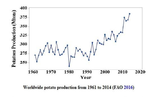
[1] | FAO (2013, 2016) Food Agriculture Organization of the United Nations Statistics Division. |
[2] |
Paleologou I, Vasiliou A, Grigorakis S, et al. (2016) Optimisation of a green ultrasound-assisted extraction process for potato peel (Solanum tuberosum) polyphenols using bio-solvents and response surface methodology. Biomass Convers Bior 6: 289-299. doi: 10.1007/s13399-015-0181-7
![]() |
[3] |
Chiellini E, Cinelli P, Chiellini F, et al. (2004) Environmentally degradable bio‐based polymeric blends and composites. Macromol Biosci 4: 218-231. doi: 10.1002/mabi.200300126
![]() |
[4] | Chang K (2019) Polyphenol antioxidants from potato peels: Extraction optimization and application to stabilizing lipid oxidation in foods. In: Proceedings of Proceedings of the National Conference on Undergraduate Research (NCUR), New York, NY, USA. |
[5] |
Nelson M (2010) Utilization and application of wet potato processing coproducts for finishing cattle. J Anim Sci 88: E133-E142. doi: 10.2527/jas.2009-2502
![]() |
[6] |
Liang S, McDonald AG, Coats ER, et al. (2014) Lactic acid production with undefined mixed culture fermentation of potato peel waste. Waste Manag 34: 2022-2027. doi: 10.1016/j.wasman.2014.07.009
![]() |
[7] |
Bhushan S, Kalia K, Sharma M, et al. (2008) Processing of apple pomace for bioactive molecules. Crit Rev Biotechnol 28: 285-296. doi: 10.1080/07388550802368895
![]() |
[8] |
Arapoglou D, Varzakas T, Vlyssides A, et al. (2010) Ethanol production from potato peel waste (PPW). Waste Manag 30: 1898-1902. doi: 10.1016/j.wasman.2010.04.017
![]() |
[9] |
Mohdaly AAA, Hassanien MFR, Mahmoud A, et al. (2013) Phenolics extracted from potato, sugar beet, and sesame processing by-products. INT J Food Prop 16: 1148-1168. doi: 10.1080/10942912.2011.578318
![]() |
[10] | Sepelev I, Galoburda R (2015) Industrial potato peel waste application in food production: A review. Res Rural Dev 1: 130-136. |
[11] | Pathak PD, Mandavgane SA, Kulkarni BD, et al. (2015) Fruit peel waste as a novel low-cost bio adsorbent. Rev Chem Eng 31: 361-381. |
[12] |
Maldonado AFS, Mudge E, Gänzle MG, et al. (2014) Extraction and fractionation of phenolic acids and glycoalkaloids from potato peels using acidified water/ethanol-based solvents. Food Res Int 65: 27-34. doi: 10.1016/j.foodres.2014.06.018
![]() |
[13] | Jeddou KB, Chaari F, Maktouf S, et al. (2016) Structural, functional, and antioxidant properties of water-soluble polysaccharides from potatoes peels. Food Chem205: 97-105. |
[14] |
Liang S, McDonald AG (2014) Chemical and thermal characterization of potato peel waste and its fermentation residue as potential resources for biofuel and bioproducts production. J Agric Food Chem 62: 8421-8429. doi: 10.1021/jf5019406
![]() |
[15] |
Liang S, Han Y, Wei L, et al. (2015) Production and characterization of bio-oil and bio-char from pyrolysis of potato peel wastes. Biomass Convers Bior 5: 237-246. doi: 10.1007/s13399-014-0130-x
![]() |
[16] | Onyeneho SN, Hettiarachchy NS (1993) Antioxidant activity, fatty acids and phenolic acids compositions of potato peels. J Sci Food Agric62: 345-350. |
[17] | Camire ME, Violette D, Dougherty MP, et al. (1997) Potato peel dietary fiber composition: Effects of peeling and extrusion cooking processes. J Agric Food Chem45: 1404-1408. |
[18] |
Camire ME, Zhao J, Violette DA, et al. (1993) In vitro binding of bile acids by extruded potato peels. J Agric Food Chem 41: 2391-2394. doi: 10.1021/jf00036a033
![]() |
[19] | Mahmood A, Greenman J, Scragg A, et al. (1998) Orange and potato peel extracts: Analysis and use as Bacillus substrates for the production of extracellular enzymes in continuous culture. Enzyme Microb Technol22: 130-137. |
[20] |
Ballesteros MN, Cabrera RM, Saucedo MS, et al. (2001) Dietary fiber and lifestyle influence serum lipids in free living adult men. J Am Coll Nutr 20: 649-655. doi: 10.1080/07315724.2001.10719163
![]() |
[21] | Lazarov K, Werman MJ (1996) Hypocholesterolaemic effect of potato peels as a dietary fibre source. Med Sci Res 24: 581-582. |
[22] |
Alonso A, Beunza JJ, Bes-Rastrollo M, et al. (2006) Vegetable protein and fiber from cereal are inversely associated with the risk of hypertension in a Spanish cohort. Arch Med Res 37: 778-786. doi: 10.1016/j.arcmed.2006.01.007
![]() |
[23] |
Erkkilä AT, Lichtenstein AH (2006) Fiber and cardiovascular disease risk: How strong is the evidence. J Cardiovasc Nurs 21: 3-8. doi: 10.1097/00005082-200601000-00003
![]() |
[24] |
Camire ME, Zhao J, Dougherty MP, et al. (1995) In Vitro binding of benzo [a] pyrene by extruded potato peels. J Agric Food Chem 43: 970-973. doi: 10.1021/jf00052a024
![]() |
[25] | Kyzas GZ, Deliyanni EA (2015) Modified activated carbons from potato peels as green environmental-friendly adsorbents for the treatment of pharmaceutical effluents. Chem Eng Res Des97: 135-144. |
[26] | Abd-El-Magied MM (1991) Effect of dietary fibre of potato peel on the rheological and organoleptic characteristics of biscuits. Egypt J Food Sci 19: 293-300. |
[27] | Al-Weshahy A, Rao V (2012) Potato peel as a source of important phytochemical antioxidant nutraceuticals and their role in human health-A review. In: Phytochemicals as Nutraceuticals-Global Approaches to Their Role in Nutrition and Health, InTech. |
[28] |
Panda SK, Mishra SS, Kayitesi E, et al. (2016) Microbial-processing of fruit and vegetable wastes for production of vital enzymes and organic acids: Biotechnology and scopes. Environ Res 146: 161-172. doi: 10.1016/j.envres.2015.12.035
![]() |
[29] |
Saldaña, MD, Valdivieso-Ramirez CS (2015) Pressurized fluid systems: Phytochemical production from biomass. J Supercrit Fluid 96: 228-244. doi: 10.1016/j.supflu.2014.09.037
![]() |
[30] | Fadel M (1999) Utilization of potato chips industry by products for the production of thermostable bacterial alpha amylase using solid state fermentation system. 1.-effect of incubation period, temperature, moisture level and inoculum size. Egypt J Microbiol. |
[31] |
Mukherjee AK, Adhikari H, Rai SK, et al. (2008) Production of alkaline protease by a thermophilic Bacillus subtilis under solid-state fermentation (SSF) condition using imperata cylindrica grass and potato peel as low-cost medium: characterization and application of enzyme in detergent formulation. Biochem Eng J 39: 353-361. doi: 10.1016/j.bej.2007.09.017
![]() |
[32] | Sharma N, Tiwari DP, Singh SK, et al. (2014) The efficiency appraisal for removal of malachite green by potato peel and neem bark: isotherm and kinetic studies. Int J Chem Environ Eng 5: 83-88. |
[33] | Prasad AGD, Pushpa HN (2007) Antimicrobial activity of potato peel waste. Asian J Microbiol Biotechnol Environ Sci 9: 559-561. |
[34] | Sharma D, Ansari MJ, Gupta S, et al. (2015) Structural characterization and antimicrobial activity of a biosurfactant obtained from Bacillus pumilus DSVP18 grown on potato peels. Jundishapur J Microbiol 8: e21257. |
[35] | Arapoglou D, Vlyssides A, Varzakas T, et al. (2009) Alternative ways for potato industries waste utilisation. In: Proceedings of Proceedings of the 11th International Conference on Environmental Science and Technolo gy, Chaina, Crete, Greece, 3-5. |
[36] | Fu BR, Sun Y, WANG YX, et al. (2013) Construction of biogas fermentation system based on feedstock of potato residue.J Northeast Agric Univ 44: 102-106. |
[37] |
Sanaei-Moghadam A, Abbaspour-Fard MH, Aghel H, et al. (2014) Enhancement of biogas production by co-digestion of potato pulp with cow manure in a CSTR system. Appl Biochem Biotechnol 173: 1858-1869. doi: 10.1007/s12010-014-0972-5
![]() |
[38] |
Liang S, McDonald AG (2015) Anaerobic digestion of pre-fermented potato peel wastes for methane production. Waste Manag 46: 197-200. doi: 10.1016/j.wasman.2015.09.029
![]() |
[39] | Datta R, Henry M (2006) Lactic acid: Recent advances in products, processes and technologies-a review. J Chem Technol Biotechnol: Int Res Process, Environ Clean Technol 81: 1119-1129. |
[40] | Priyanga K, Reji A, Bhagat JK, et al. (2016) Production of organic manure from potato peel waste. Int J Chem Tech Res 9: 845-847. |
[41] | Pandit N, Ahmad N, Maheshwari S, et al. (2012) Vermicomposting biotechnology an eco-loving approach for recycling of solid organic wastes into valuable biofertilizers. J Biofertil Biopestic 3: 1-8. |
[42] | Muhondwa J, Martienssen M, Burkhardt M, et al. (2015) Feasibility of anaerobic digestion of potato peels for biogas as mitigation of greenhouse gases emission potential. Int J Environ Res 9: 481-488 |
[43] |
Tiwari V, Maji S, Kumar S, et al. (2016) Use of kitchen waste based bio-organics for strawberry (Fragaria x ananassa Duch) production. Afr J Agric Res 11: 259-265. doi: 10.5897/AJAR2015.10349
![]() |
[44] |
Chintagunta AD, Jacob S, Banerjee R, et al. (2016) Integrated bioethanol and biomanure production from potato waste. Waste Manag 49: 320-325. doi: 10.1016/j.wasman.2015.08.010
![]() |
[45] |
Shukla J, Kar R (2006) Potato peel as a solid state substrate for thermostable α-amylase production by thermophilic Bacillus isolates. World J Microb Biot 22: 417-422. doi: 10.1007/s11274-005-9049-5
![]() |
[46] | Jadhav SA, Kataria PK, Bhise KK, et al. (2013) Amylase production from potato and banana peel waste. Int J Curr Microbiol App Sci 2: 410-414. |
[47] | Mabrouk ME, El Ahwany AM (2008) Production of 946-mannanase by Bacillus amylolequifaciens 10A1 cultured on potato peels. Afr J Biotechnol 7: 1123-1128. |
[48] |
Dos Santos TC, Gomes DPP, Bonomo RCF, et al. (2012) Optimisation of solid state fermentation of potato peel for the production of cellulolytic enzymes. Food Chem 133: 1299-1304. doi: 10.1016/j.foodchem.2011.11.115
![]() |
[49] |
Mukherjee S, Bandyopadhayay B, Basak B, et al. (2012) An improved method of optimizing the extraction of polyphenol oxidase from potato (Solanum tuberosum L.) Peel. Not Sci Biol 4: 98-107. doi: 10.15835/nsb417186
![]() |
[50] |
Niphadkar SS, Vetal MD, Rathod VK, et al. (2015) Purification and characterization of polyphenol oxidase from waste potato peel by aqueous two-phase extraction. Prep Biochem Biotechnol 45: 632-649. doi: 10.1080/10826068.2014.940970
![]() |
[51] | Da Silva Batista M, Guimarães CO, Marra LC, et al. (2015) Bio-oil production from waste potato peel and rice hush. Rev Eletrônica Gest Educ Tecnol 19: 220-227. |
[52] |
Izmirlioglu G, Demirci A (2012) Ethanol production from waste potato mash by using Saccharomyces cerevisiae. Appl Sci 2: 738-753. doi: 10.3390/app2040738
![]() |
[53] | Afsar N, Özgür E, Gürgan M, et al. (2011) Hydrogen productivity of photosynthetic bacteria on dark fermenter effluent of potato steam peels hydrolysate. Int J Hydrogen Energ36: 432-438. |
[54] |
Panagiotopoulos IA, Karaoglanoglou LS, Koullas DP, et al. (2015) Technical suitability mapping of feedstocks for biological hydrogen production. J Clean Prod 102: 521-528. doi: 10.1016/j.jclepro.2015.04.055
![]() |
[55] |
Im HW, Suh BS, Lee SU, et al. (2008) Analysis of phenolic compounds by high-performance liquid chromatography and liquid chromatography/mass spectrometry in potato plant flowers, leaves, stems, and tubers and in home-processed potatoes. J Agric Food Chem 56: 3341-3349. doi: 10.1021/jf073476b
![]() |
[56] | Lee J, Finn CE (2007) Anthocyanins and other polyphenolics in American elderberry (Sambucus canadensis) and European elderberry (S. nigra) cultivars. J Sci Food Agric87: 2665-2675. |
[57] | Rodríguez-Meizoso I, Marin FR, Herrero M, et al. (2006) Subcritical water extraction of nutraceuticals with antioxidant activity from oregano. Chemical and functional characterization. J Pharmaceut Biomed 41: 1560-1565. |
[58] |
Yeung YY, Hong S, Corey EJ, et al. (2006) A short enantioselective pathway for the synthesis of the anti-influenza neuramidase inhibitor oseltamivir from 1,3-butadiene and acrylic acid. J Am Chem Soc 128: 6310-6311. doi: 10.1021/ja0616433
![]() |
[59] |
Mansour EH, Khalil AH (2000) Evaluation of antioxidant activity of some plant extracts and their application to ground beef patties. Food Chem 69: 135-141. doi: 10.1016/S0308-8146(99)00234-4
![]() |
[60] |
Kanatt SR, Chander R, Radhakrishna P, et al. (2005) Potato peel extract a natural antioxidant for retarding lipid peroxidation in radiation processed lamb meat. J Agric Food Chem 53: 1499-1504. doi: 10.1021/jf048270e
![]() |
[61] |
Formanek Z, Lynch A, Galvin K, et al. (2003) Combined effects of irradiation and the use of natural antioxidants on the shelf-life stability of overwrapped minced beef. Meat Sci 63: 433-440. doi: 10.1016/S0309-1740(02)00063-3
![]() |
[62] |
Mohdaly AA, Sarhan MA, Smetanska I, et al. (2010) Antioxidant properties of various solvent extracts of potato peel, sugar beet pulp and sesame cake. J Sci Food Agric 90: 218-226. doi: 10.1002/jsfa.3796
![]() |
[63] | Rommi K, Rahikainen J, Vartiainen J, et al. (2016) Potato peeling costreams as raw materials for biopolymer film preparation. J Appl Polym Sci 133: 1-11. |
[64] |
Nara K, Miyoshi T, Honma T, et al. (2006) Antioxidative activity of bound-form phenolics in potato peel. Biosci Biotechnol Biochem 70: 1489-1491. doi: 10.1271/bbb.50552
![]() |
[65] |
Arun K, Chandran J, Dhanya R, et al. (2015) Comparative evaluation of antioxidant and antidiabetic potential of peel from young and matured potato. Food Biosci 9: 36-46. doi: 10.1016/j.fbio.2014.10.003
![]() |
[66] | Shimoi K, Okitsu A, Green M, et al. (2001) Oxidative DNA damage induced by high glucose and its suppression in human umbilical vein endothelial cells. Mutat Res-Fund Mol M 480: 371-378. |
[67] | Singh N, Kamath V, Rajini P, et al. (2005) Attenuation of hyperglycemia and associated biochemical parameters in STZ-induced diabetic rats by dietary supplementation of potato peel powder. Clin Chim Acta353: 165-175. |
[68] | El Bohi KM, Hashimoto Y, Muzandu K, et al. (2009) Protective effect of Pleurotus cornucopiae mushroom extract on carbon tetrachloride-induced hepatotoxicity. Jpn J Vet Res 57: 109-118. |
[69] |
Singh N, Rajini P (2008) Antioxidant-mediated protective effect of potato peel extract in erythrocytes against oxidative damage. Chem Biol Interact 173: 97-104. doi: 10.1016/j.cbi.2008.03.008
![]() |
[70] |
Jaeschke H, Gores GJ, Cederbaum AI, et al. (2002) Mechanisms of hepatotoxicity. Toxicol Sci 65: 166-176. doi: 10.1093/toxsci/65.2.166
![]() |
[71] |
Tasaduq S, Singh K, Sethi S, et al. (2003) Hepatocurative and antioxidant profile of HP-1, a polyherbal phytomedicine. Hum Exp Toxicol 22: 639-645. doi: 10.1191/0960327103ht406oa
![]() |
[72] |
Mohammed NMS, Salim HAM (2017) Adsorption of Cr (Vi) ion from aqueous solutions by solid waste of potato peels. Sci J Uni Zakho 5: 254-258. doi: 10.25271/2017.5.3.392
![]() |
[73] |
Bibi S, Farooqi A, Yasmin A, et al. (2017) Arsenic and fluoride removal by potato peel and rice husk (PPRH) ash in aqueous environments. Int J Phytoremediat 19: 1029-1036. doi: 10.1080/15226514.2017.1319329
![]() |
[74] | Guechi EK, Hamdaoui O (2016) Evaluation of potato peel as a novel adsorbent for the removal of Cu (Ⅱ) from aqueous solutions: equilibrium, kinetic, and thermodynamic studies. Desalin Water Treat57: 10677-10688. |
[75] |
Kyzas GZ, Deliyanni EA, Matis KA, et al. (2016) Activated carbons produced by pyrolysis of waste potato peels: Cobalt ions removal by adsorption. Colloids Surf, A 490: 74-83. doi: 10.1016/j.colsurfa.2015.11.038
![]() |
[76] | Mahale KK, Mokhasi HR, Ashoka H, et al. (2016) Biosorption of nickel (Ⅱ) from aqueous solutions using potato peel. Res J Chem Environ Sci 4: 96-101. |
[77] | Mutongo F, Kuipa O, Kuipa PK, et al. (2014) Removal of Cr (VI) from aqueous solutions using powder of potato peelings as a low cost sorbent. Bioinorg Chem Appl 2014: 1-7. |
1. | Yanbing Wang, Daniel B. Work, Estimation for heterogeneous traffic using enhanced particle filters, 2022, 18, 2324-9935, 568, 10.1080/23249935.2021.1881186 | |
2. | Zlatinka Dimitrova, Flows of Substances in Networks and Network Channels: Selected Results and Applications, 2022, 24, 1099-4300, 1485, 10.3390/e24101485 | |
3. | M. L. Delle Monache, J. Sprinkle, R. Vasudevan, D. Work, 2019, Autonomous vehicles: From vehicular control to traffic contro, 978-1-7281-1398-2, 4680, 10.1109/CDC40024.2019.9029535 | |
4. | Yanbing Wang, Daniel B. Work, 2019, Heterogeneous traffic estimation with particle filtering, 978-1-5386-7024-8, 2551, 10.1109/ITSC.2019.8917248 | |
5. | Joel C. de Goma, Lourd Andre B. Ammuyutan, Hans Luigi S. Capulong, Katherine P. Naranjo, Madhavi Devaraj, 2019, Vehicular Obstruction Detection In The Zebra Lane Using Computer Vision, 978-1-7281-0851-3, 362, 10.1109/IEA.2019.8715022 | |
6. | Maria Laura Delle Monache, Sean T. McQuade, Hossein Nick Zinat Matin, Derek A. Gloudemans, Yanbing Wang, George L. Gunter, Alexandre M. Bayen, Jonathan W. Lee, Benedetto Piccoli, Benjamin Seibold, Jonathan M. Sprinkle, Daniel B. Work, Modeling, Monitoring, and Controlling Road Traffic Using Vehicles to Sense and Act, 2025, 8, 2573-5144, 211, 10.1146/annurev-control-030123-015145 |
Parameter | Interpretation | Standard value | Range | Source |
r | Recruitment rate of plant | 0.015(day−1) | 0–0.025 | Assumed |
α | Plant roguing rate | 0.003(day−1) | 0–0.033 | [19] |
g | Plant loss/harvesting rate | 0.003(day−1) | 0.002–0.004 | [19] |
μ | Recruitment rate of vector | 400(day−1) | 0–2500 | Assumed |
c | Vector mortality | 0.12(day−1) | 0.06–0.18 | [19] |
k1 | Infection rate | 0.008(vector−1day−1) | 0.002–0.032 | [19] |
k2 | Acquisition rate | 0.008(plant−1day−1) | 0.002–0.032 | [19] |