Loading [MathJax]/jax/output/SVG/jax.js
Research article Special Issues

Bifurcation analysis in a singular Beddington-DeAngelis predator-prey model with two delays and nonlinear predator harvesting

  • In this paper, a differential algebraic predator-prey model including two delays, Beddington-DeAngelis functional response and nonlinear predator harvesting is proposed. Without considering time delay, the existence of singularity induced bifurcation is analyzed by regarding economic interest as bifurcation parameter. In order to remove singularity induced bifurcation and stabilize the proposed system, state feedback controllers are designed in the case of zero and positive economic interest respectively. By the corresponding characteristic transcendental equation, the local stability of interior equilibrium and existence of Hopf bifurcation are discussed in the different case of two delays. By using normal form theory and center manifold theorem, properties of Hopf bifurcation are investigated. Numerical simulations are given to demonstrate our theoretical results.

    Citation: Xin-You Meng, Yu-Qian Wu. Bifurcation analysis in a singular Beddington-DeAngelis predator-prey model with two delays and nonlinear predator harvesting[J]. Mathematical Biosciences and Engineering, 2019, 16(4): 2668-2696. doi: 10.3934/mbe.2019133

    Related Papers:

    [1] Yufeng Li, Chengcheng Liu, Weiping Zhao, Yufeng Huang . Multi-spectral remote sensing images feature coverage classification based on improved convolutional neural network. Mathematical Biosciences and Engineering, 2020, 17(5): 4443-4456. doi: 10.3934/mbe.2020245
    [2] Ting Yao, Farong Gao, Qizhong Zhang, Yuliang Ma . Multi-feature gait recognition with DNN based on sEMG signals. Mathematical Biosciences and Engineering, 2021, 18(4): 3521-3542. doi: 10.3934/mbe.2021177
    [3] Tao Zhang, Hao Zhang, Ran Wang, Yunda Wu . A new JPEG image steganalysis technique combining rich model features and convolutional neural networks. Mathematical Biosciences and Engineering, 2019, 16(5): 4069-4081. doi: 10.3934/mbe.2019201
    [4] Zhangjie Wu, Minming Gu . A novel attention-guided ECA-CNN architecture for sEMG-based gait classification. Mathematical Biosciences and Engineering, 2023, 20(4): 7140-7153. doi: 10.3934/mbe.2023308
    [5] Xianli Liu, Yongquan Zhou, Weiping Meng, Qifang Luo . Functional extreme learning machine for regression and classification. Mathematical Biosciences and Engineering, 2023, 20(2): 3768-3792. doi: 10.3934/mbe.2023177
    [6] Sakorn Mekruksavanich, Wikanda Phaphan, Anuchit Jitpattanakul . Epileptic seizure detection in EEG signals via an enhanced hybrid CNN with an integrated attention mechanism. Mathematical Biosciences and Engineering, 2025, 22(1): 73-105. doi: 10.3934/mbe.2025004
    [7] Jia-Gang Qiu, Yi Li, Hao-Qi Liu, Shuang Lin, Lei Pang, Gang Sun, Ying-Zhe Song . Research on motion recognition based on multi-dimensional sensing data and deep learning algorithms. Mathematical Biosciences and Engineering, 2023, 20(8): 14578-14595. doi: 10.3934/mbe.2023652
    [8] Zhigao Zeng, Cheng Huang, Wenqiu Zhu, Zhiqiang Wen, Xinpan Yuan . Flower image classification based on an improved lightweight neural network with multi-scale feature fusion and attention mechanism. Mathematical Biosciences and Engineering, 2023, 20(8): 13900-13920. doi: 10.3934/mbe.2023619
    [9] Haifeng Song, Weiwei Yang, Songsong Dai, Haiyan Yuan . Multi-source remote sensing image classification based on two-channel densely connected convolutional networks. Mathematical Biosciences and Engineering, 2020, 17(6): 7353-7377. doi: 10.3934/mbe.2020376
    [10] Xiaoguang Liu, Yubo Wu, Meng Chen, Tie Liang, Fei Han, Xiuling Liu . A double-channel multiscale depthwise separable convolutional neural network for abnormal gait recognition. Mathematical Biosciences and Engineering, 2023, 20(5): 8049-8067. doi: 10.3934/mbe.2023349
  • In this paper, a differential algebraic predator-prey model including two delays, Beddington-DeAngelis functional response and nonlinear predator harvesting is proposed. Without considering time delay, the existence of singularity induced bifurcation is analyzed by regarding economic interest as bifurcation parameter. In order to remove singularity induced bifurcation and stabilize the proposed system, state feedback controllers are designed in the case of zero and positive economic interest respectively. By the corresponding characteristic transcendental equation, the local stability of interior equilibrium and existence of Hopf bifurcation are discussed in the different case of two delays. By using normal form theory and center manifold theorem, properties of Hopf bifurcation are investigated. Numerical simulations are given to demonstrate our theoretical results.


    Deep learning becomes one of the most important technologies in the field of artificial intelligence [1,2,3]. CNN is the most representative model of deep learning [4]. In 1989, Yann LeCun [5] proposes CNN model and applies CNN to handwritten character recognition. Yoshua Bengio presents the Probabilistic models of sequences and proposes generative adversarial networks [6]. Geoffrey Hinton et al. present a deep brief net [7] and apply CNN in Image Net game. The advantages of CNN against traditional methods can be summarized as follows [4].

    (1) Hierarchical feature representation.

    (2) Compared with traditional shallow models, a deeper architecture provides an exponentially increased expressive capability.

    (3) The architecture of CNN provides an opportunity to optimize several related tasks together.

    (4) Benefiting from the large learning capacity of CNNs, some classical computer vision challenges can be recast as high-dimensional data transform problems and solved from a different viewpoint.

    Due to these advantages, CNN has been widely applied into many research fields [8,9,10,11,12,13,14]. However, the CNN has some disadvantages. Many Parameters need to be adjusted in CNN. It needs many training samples and the GPU is preferred for training CNN.

    Extreme learning machine (ELM) [15] is a kind of feed-forward neural network in essence. ELM generates input layer weights and bias values at random, directly solves the least square solution of the output weights, and obtains the final training model at the same time. ELM has the advantages such as no iterative calculation, fast learning speed and strong generalization ability. Many scholars pay close attention to ELM and have achieved good results [16,17,18,19,20]. A fast kernel ELM combining the conjugate gradient method (CG-KELM) is presented in [16] and the kernel ELM is applied in image restoration. In [17], the paper further studies ELM for classification in the aspect of the standard optimization method and extends ELM to a specific type of "generalized" single-hidden layer feedforward networks-support vector network. An improved meta-learning model of ELM is proposed in [18]. Chunmei He et al. [19] propose a fast learning algorithm for the regular fuzzy neural network based on ELM which has good performance and approximation ability. Since ELM is based on the principle of empirical risk minimization which may lead to over-fitting problem. In [20], the scholars combine the structural risk minimization theory and weighted least square method and present RELM. RELM considers both the structural risk and the empirical risk and balances the two risks using the risk ratio parameter. RELM is widely used in the fields of classification, regression and prediction. RELM has the advantage of fast learning speed and further improves the generalization performance of ELM.

    Motivated by the remarkable success of CNN and RELM, RELM is introduced into CNN and an effective classifier CNN-RELM is proposed in this paper. In CNN-RELM, CNN can extract the deep feature of the input, while RELM have fast learning speed and good generalized ability to acquire better recognized accuracy. The rest paper is organized as follows. Section 2 introduces the basic theory of CNN, ELM and RELM. The CNN-RELM model and learning algorithm are presented in section 3. The experiment simulations show the excellent performance of the CNN-RELM in section 4. Section 5 summarizes the study and discusses the future work.

    A typical CNN is simply introduced here. The CNN topological model is shown in Figure 1.

    Figure 1.  CNN topological model. The CNN has two convolution layers C1 and C3, two pooling layers S2 and S4 and the fully connected layer.

    In the CNN, the convolution layer and pooling layer extract the features and input into the fully connected layer to obtain the classification results. The feature extraction process is as follows.

    In the convolution layer, convolution is performed on the input, and the output is

    xlj=f(iMjxl1iwlij+blj) (1)

    where Mj is the input set and b is the bias of the convolution layer.

    The gradient of the convolution layer is defined by δlj=βl+1j(f(ulj)up(δl+1j)).

    The output of the pooling layer is

    xlj=f(βljdown(xl1i)+blj) (2)

    where down() is the pooling function, b is the bias, and β is the weight.

    In the fully connected layer, the output of the l-th layer is xl=f(ul), where ul=wlxl1+bl, wl is the weight and bl is the bias of the l-th layer.

    We simply introduce ELM and RELM. For more details, please refer to [15,20]. The topology of ELM is shown in Figure 2.

    Figure 2.  The topology of ELM. In Figure 2, ELM has n input layer nodes, l hidden layer nodes and m output nodes. xj=[xj1,xj2,,xjn]TRn is the input, wi is the weight, bi is the bias, oj=[oj1,oj2,,ojm]TRm is the actual output and β is the output weight matrix between the hidden layer and the output layer.

    Different from other feed-forward neural networks, the input weight wi and bias bi of the ELM are generated randomly in the training. After the input sample set (xj,yj) is processed by the hidden layer neurons, the hidden layer output matrix H of ELM can be fixed. The goal of ELM is to adjust the weight ˆβ satisfying the following equation.

    HˆβY=minβHβY (3)

    where β=[βT1,,βTl]Tl×m, Y=[yT1,,yTN]TN×m is the expected output and

    H(w1,,wl,b1,,bl,x1,,xn)=[g(w1x1+b1)g(wlx1+bl)g(w1xn+b1)g(wlxn+bl)]l×n. (4)

    The solution of Eq (3) is the least normal square solution as follows.

    ˆβ=H+Y, (5)

    where H+ is the Moore-Penrose generalized inverse matrix.

    ELM only considers the empirical risk and doesn't consider the structural risk. ELM directly calculates the least squares solution, and users can't make fine-tuning according to the characteristics of the database, these results in poor control ability and over-fitting problems. Therefore, the structural risk minimization theory is introduced into ELM, and RELM is proposed [20]. The RELM model is as follows. When γ, the RELM degenerates into the ELM, that is, ELM is a special case of the RELM.

    argβminE(W)=argβminE(0.5β2+0.5γε2),s.t.li=1βig(wixj+bi)yj=εj,j=1,,n. (6)

    where β2 is the structural risk, ε is the error, ε2 is the empirical risk, γ is the proportion parameters to balance empirical risk and structural risk. The Eq (6) is a conditional extreme problem, which is solved by converting Lagrange equation into an unconditional extreme problem as follows.

    (β,ε,α)=γ2ε2+12β2nj=1αj(g(wixj+bj)yjεj)=γ2ε2+12β2α(HβYε) (7)

    where αjRm(j=1,,n) is Lagrange operator. Let the gradient of the Lagrange equation be 0 and compute the weight β as follows.

    β=(Iγ+HTH)+HTY. (8)

    In this section, the CNN-RELM model and learning algorithm are presented. In CNN-RELM, the convolutional hidden layer and the pooling layer in CNN extract deep features from the original input and then RELM are used for feature classification. The CNN-RELM model is changed in the two steps of training period. And in testing period, there is no fully connected layer in CNN which is replaced by the RELM.A trained CNN-RELM used for testing is as in Figure 3. The training of CNN-RELM model is divided into two steps: The training of CNN and the merger of CNN and RELM. These two steps are presented in detail as follows.

    Figure 3.  The trained CNN-RELM for testing. In CNN, input is the sample image, C1 and C3 are the convolutional layers, S2 and S4 are the pooling layers. In RELM, x is the input, w is the weight between input-layer and hidden-layer, β is the weight between hidden-layer and output-layer, and y is the output.

    In this step, the CNN model is trained. The CNN model in this step is as in Figure 4. The related parameters in CNN are adjusted by the gradient descent method according to the errors between the actual output and the expected output. The training of the CNN stops if the minimum error reaches or the maximum number of iterations reaches. Then the CNN is saved for the next step.

    Figure 4.  The topology of CNN model. In CNN, C1andC3 are two convolution layers, S2andS4 are two pooling layers, and C5 is the fully connected layer.

    The feature map in the CNN is adjusted as follows.

    (a) If the m-th layer is a convolution layer, the n-th feature map is

    xlj=f(xm1iMnxm1ikmin+bmn) (9)

    where Mn is the input set; f is a nonlinear active function; kmin is the convolution kernel; bmn is bias.

    (b) If the m-th layer is a pool layer, its n-th feature map is

    xmn=f(wmndown(xm1n)+bmn) (10)

    where wmn is weight, bmn is bias and down() is pooling function. The two pooling methods: The max pooling and the mean pooling are used here.

    In this step, we firstly acquire the RELM which is optimized by genetic algorithm. And then the convolutional layers and pooling layers of the CNN is fixed while the full-connected layer of the CNN is replaced by the RELM. The topology of RELM is also shown as in Figure 3. The optimal risk ratio parameters γ in the RELM are optimized by genetic algorithm. The RELM mathematical model is the same as Eq (6). The weight β is computed by Eq (8). The fully-connected layer of CNN is replaced by the RELM. In other words, the feature images trained by CNN are considered as the input of RELM, and the desired classification results are obtained through RELM. The role of RELM is to act as a classifier in CNN-RELM model.

    The learning algorithm of CNN-RELM is outlined in Algorithm 1. The learning algorithm flow chart of CNN-RELM is shown as in Figure 5.

    Figure 5.  The learning algorithm flow chart of CNN-RELM. CNN-RLEM is divided into two parts: CNN and RELM. The related parameters in CNN are adjusted by the gradient descent method according to the errors between the actual output and the expected output. The training process stops if the minimum error reaches or the maximum number of iterations reaches. Then the main part of the CNN is fixed except that the full-connected layer of the CNN is replaced by RELM. The optimal risk ratio parameters γ in the RELM are optimized by genetic algorithm.

    Algorithm 1

    Step 1. Initialize the CNN parameters, expected target and maximum iteration times.

    Step 2. Compute the actual output of the network by Eqs (9), (10).

    Step 3. If the predetermined target precision reaches or the maximum number of iterations reaches, then go to Step 5, else go to Step 4.

    Step 4. Adjust the parameters of CNN by the gradient descent method and go to Step 2.

    Step 5. Initialize RELM. Randomly initialize the weights and biases. Get the regularized parameters by GA.

    Step 6. Let the feature vectors obtained by CNN into RELM and Compute β by Eq (8).

    Step 7. Save the CNN-RELM and classify by the CNN-RELM.

    In this section, we present the face recognition experiment to verify the feasibility of CNN-RELM and compare it with RELM and CNN. The impacts of different pooling methods and different number of training samples on the performance of CNN-RELM are also presented.

    Two face databases: ORL and NUST are used in the simulations. The detailed database information is shown in Table 1. The ORL face database is founded by the Olivetti research laboratory in Cambridge, England. The ORL face database can be downloaded in the following website: http://www.cl.cam.ac.uk/research/dtg/attarchive/facedatabase.html. The NUST face database is made by Nanjing University of Science and Technology, China.

    Table 1.  Face databases information.
    databases classes features number of samples remarks
    ORL 40 10 400 These include changes in facial expressions, minor changes in posture, and changes in scale within 20%.
    NUST 96 10 216 It mainly includes the change of face's different pose.

     | Show Table
    DownLoad: CSV

    The experimental execution environment is as follows. Software environment: Matlab-R2014a. Operation system: Windows 8. Hardware environment: Dell PC. CPU: Intel(R) Core(TM) i5-6500 CPU @ 3.20GHz. Hard disk: Seagate ST500DM002-1SB10A (500 GB /7200 rpm). Memory: 32 GB (Samsung DDR4 2666MHz).

    To evaluate the performance of CNN-RELM, some simulations on the ORL face databases are given. In training of the CNN, there are two convolution layers: C1, C3 and two pool layers: S2, S4. The convolution kernel of convolution layer C1 and C3 are all set as 9×9 matrix. In pooling layer S2 and S4, max-pooling is used and the window size is 3×3. The gradient descent algorithm is used to train the CNN. The error function of CNN in the training is shown in Figure 6. As the number of iterations increases, the training error gradually decreases.

    Figure 6.  Training error curve of CNN.

    After the CNN is trained, the fully connected layer is replaced by RELM for classification. The feature images obtained by the pooling layer S4 are converted into column vectors and stored in matrix. Moreover, the RELM model is used for classification. When initializing RELM, we obtain the input weight and bias in a random way. At the same time, we use the optimal risk ratio parameter mentioned in [21], and the hidden layer nodes are set to 200. The test results are shown in Figure 7. The experimental results show that the proposed algorithm is feasible in face recognition.

    Figure 7.  Face recognition results of CNN-RELM.

    In this section, we compare the performances of CNN-RELM, RELM and CNN in face recognition experiments. The parameters in the CNN and the risk ratio parameter of RELM are similar to that in [21]. Two standard face databases: ORL and NUST as in Table 1 are used in the comparative experiments. In the experiment, we select seven images of each person as training samples, and the remaining three images as test samples. All hidden layer node number of neural networks is set to 200. The recognition results of the three algorithms are shown in Table 2.

    Table 2.  Comparison of different methods in face recognition. Specially point out: The bold fonts are the results of our method.
    databases methods division of sample sets classification accuracy (%)
    training samples test samples
    ORL RELM
    CNN
    CNN-RELM
    280
    280
    280
    120
    120
    120
    91.67
    90.00
    96.67
    NUST RELM
    CNN
    CNN-RELM
    672
    672
    672
    288
    288
    288
    89.58
    88.54
    96.88

     | Show Table
    DownLoad: CSV

    As seen from Table 2, the CNN-RELM model proposed in this paper has the best recognition accuracy. In next section, an experiment is given to study the influence of different pooling methods and number of the training sample on CNN-RELM.

    In order to evaluate how different pooling methods and different training samples impact on the performance of the CNN-RELM, the experiment is conducted in this section. The ORL face database is selected here. The parameters of the CNN-RELM model are selected as the same as those in section 4.2. The pooling method respectively uses Max-pooling, Average-pooling, Stochastic-pooling and Lp-pooling. Figures 47 are selected for each class's training samples and the rest pictures are taken as test samples. The experimental results are shown in Table 3 and Figure 8.

    Table 3.  Face recognition results of CNN-RELM with different pooling methods and different number of training samples. The highest recognition rate marks in bold fonts.
    methods training samples
    4 5 6 7
    Max-pooling 83.75 88.00 94.37 96.67
    Average-pooling 84.17 92.00 96.25 97.50
    Stochastic-pooling 83.75 89.50 95.00 96.67
    Lp-pooling 84.58 92.50 96.88 98.33

     | Show Table
    DownLoad: CSV
    Figure 8.  Face recognition results of different pooling methods. In the figure, the abscissa represents the number of training samples for each category, and the ordinate is the corresponding recognition rate. For example, the abscissa value 4 indicates that 4 pictures are selected as training samples and the remaining ones are used as test samples. The ordinate is the corresponding recognition rate.

    By the experiment in Figures 6 and 7, it's known that the CNN-RELM is feasible in classification. From Table 2, we can concluded that the CNN-RELM outperform CNN and RELM in classification. The CNN-RELM model combines CNN with RELM and overcomes the deficiency of the two models. The CNN-RELM can also be used in other application tasks such as remote sensing and object shape reconstruction and the process is similar to that of classification.

    From Table 3 and Figure 8, we can see that the recognition rate increase at the same pooling strategy as the selected training samples increase. When the same number of training samples is selected, the Lp pooling strategy has the highest recognition rate. The recognition rate corresponding to the average pooling strategy, the statistics pooling strategy and the maximum pooling strategy are sequentially reduced.

    Seen from Figure 8, the selection of different pooling methods has an impact on the performance of CNN-RELM. In practical applications, the selection of appropriate pooling methods according to the actual situation of data is conducive to achieving better application results.

    An effective classifier CNN-RELM is proposed in this paper. Firstly, the CNN-RELM trains the convolutional neural network using the gradient descent method until the learning target accuracy reaches. Then the fully connected layer of CNN is replaced by RELM optimized by genetic algorithm and the rest layers of the CNN remain unchanged. A series of experiments conducted on ORL and NUST databases show that the CNN-RELM outperforms CNN and RELM in classification and demonstrate the efficiency and accuracy of the proposed CNN-RELM model. Meanwhile, we also verify that the selection of different pooling methods has an impact on the performance of CNN-RELM. When the same number of training samples is selected, the pooling strategy has the highest recognition rate. In practical applications, the selection of appropriate pooling methods according to the actual situation of data is conducive to achieving better application results. Due to the uniting of CNN and RELM, CNN-RELM have the advantages of CNN and RELM and it is easier to learn and faster in testing. The future work includes improve the generalized ability and further reduce the training time.

    This work is supported by the National Natural Science Foundation of China (Grant No. 61402227), the Natural Science Foundation of Hunan Province (No.2019JJ50618) and the project of Xiangtan University (Grant No. 11kz/kz08055). This work is also supported by the key discipline of computer science and technology in Hunan province, China.

    The authors declare there is no conflict of interest.


    [1] M. Kot, Elements of Mathematical Biology, Cambridge University Press, Cambridge, 2001.
    [2] S. Levin, T. Hallam and J. Cross, Applied Mathematical Ecology, Springer, New York, 1990.
    [3] R. May, Stability and Complexity in Model Ecosystems, Princeton University Press, Princeton, 1993.
    [4] C. Ji, D. Jing and N. Shi, A note on a predator-prey model with modified Leslie-Gower and Holling-type II schemes with stochastic perturbatio, J. Math. Anal. Appl., 377 (2011), 435–440.
    [5] T. Kar and H. Matsuda, Global dynamics and controllability of a harvested prey-predator system with Holling type III functional response, Nonlinear Anal. Hybrid Syst., 1 (2007), 59–67.
    [6] X. Meng, J. Wang, H. Huo, Dynamical behaviour of a nutrient-plankton model with Holling type IV, delay, and harvesting, Discrete Dyn. Nat. Soc., 2018 (2018), Article ID 9232590.
    [7] X. Meng, H. Huo, H. Xiang, et al., Stability in a predator-prey model with Crowley-Martin function and stage structure for prey, Appl. Math. Comput., 232 (2014), 810–819.
    [8] W. Yang, Diffusion has no influence on the global asymptotical stability of the Lotka-Volterra pre-predator model incorporating a constant number of prey refuges, Appl. Math. Comput., 223 (2013), 278–280.
    [9] Y. Zhu and K.Wang, Existence and global attractivity of positive periodic solutions for a predatorprey model with modified Leslie-Gower Holling-type II schemes, J. Math. Anal. Appl., 384 (2011), 400–408.
    [10] J. Liu, Dynamical analysis of a delayed predator-prey system with modified Leslie-Gower and Beddington-DeAngelis functional response, Adv. Difference Equ., 2014 (2014), 314–343.
    [11] X. Liu and Y. Wei, Dynamics of a stochastic cooperative predator-prey system with Beddington- DeAngelis functional response, Adv. Difference Equ., 2016 (2016), 21–39.
    [12] C. Li, X. Guo and D. He, An impulsive diffusion predator-prey system in three-species with Beddington-DeAngelis response, J. Appl. Math. Comput., 43 (2013), 235–248.
    [13] T. Ivanov and N. Dimitrova, A predator-prey model with generic birth and death rates for the predator and Beddington-DeAngelis functional response, Math. Comput. Simulat., 133 (2017), 111–123.
    [14] Q. Meng and L. Yang, Steady state in a cross-diffusion predator-prey model with the Beddington- DeAngelis functional response, Nonlinear Anal.: Real World Appl., 45 (2019), 401–413.
    [15] W. Liu, C. Fu and B. Chen, Hopf bifurcation and center stability for a predator-prey biological economic model with prey harvesting, Commun. Nonlinear Sci. Numer. Simul., 17 (2012), 3989– 3998.
    [16] F. Conforto, L. Desvillettes and C. Soresina, About reaction-diffusion systems involving the Holling-type II and the Beddington-DeAngelis functional responses for predator-prey models, Nonlinear Differ. Equ. Appl., 25 (2018), 24.
    [17] X. Sun, R. Yuan and L. Wang, Bifurcations in a diffusive predator-prey model with Beddington- DeAngelis functional response and nonselective harvesting, J. Nonlinear Sci., 29 (2019), 287–318.
    [18] J. Beddington, Mutual interference between parasites or predators and its effect on searching efficiency, J. Anim. Ecol., 44 (1975), 331–340.
    [19] D. DeAngilis, R. Goldstein and R. Neill, A model for tropic interaction, Ecology, 56 (1975), 881–892.
    [20] H. Freedman, Deterministic Mathematical Models in Population Ecology, Marcel Dekker, New York, 1980.
    [21] G. Seifert, Asymptotical behavior in a three-component food chain model, Nonlinear Anal. Theory Methods Appl., 32 (1998), 749–753.
    [22] C. Liu, Q. Zhang, X. Zhang, et al., Dynamical behavior in a stage-structured differential-algebraic prey-predator model with discrete time delay and harvesting, J. Comput. Appl. Math., 231 (2009), 612–625.
    [23] X. Meng, H. Huo, X. Zhang, et al., Stability and hopf bifurcation in a three-species system with feedback delays, Nonlinear Dyn., 64 (2011), 349–364.
    [24] X. Meng and Y. Wu, Bifurcation and control in a singular phytoplankton-zooplankton-fish model with nonlinear fish harvesting and taxation, Int. J. Bifurcat. Chaos, 28 (2018), 1850042(24 pages).
    [25] H. Xiang, Y. Wang and H. Huo, Analysis of the binge drinking models with demographics and nonlinear infectivity on networks, J. Appl. Anal. Comput., 8 (2018), 1535–1554.
    [26] K. Chakraborty, M. Chakraboty and T. Kar, Bifurcation and control of a bioeconomic model of a prey-predator system with a time delay, Nonlinear Anal. Hybrid Syst., 5 (2011), 613–625.
    [27] W. Liu, C. Fu and B. Chen, Hopf birfucation for a predator-prey biological economic system with Holling type II functional response, J. Franklin Inst., 348 (2011), 1114–1127.
    [28] G. Zhang, B. Chen, L. Zhu, et al., Hopf bifurcation for a differential-algebraic biological economic system with time delay, Appl. Math. Comput, 218 (2012), 7717–7726.
    [29] T. Faria, Stability and bifurcation for a delayed predator-prey model and the effect of diffusion, J. Math. Anal. Appl., 254 (2001), 433–463.
    [30] G. Zhang, Y. She and B. Chen, Hopf bifurcation of a predator prey system with predator harvesting and two delays, Nonlinear Dyn., 73 (2013), 2119–2131.
    [31] J. Zhang, Z. Jin, J. Yan, et al., Stability and Hopf bifurcation in a delayed competition system, Nonlinear Anal. Theory Methods Appl., 70 (2009), 658–670.
    [32] Z. Lajmiri, R. K. Ghaziani and I. Orak, Bifurcation and stability analysis of a ratio-dependent predator-prey model with predator harvesting rate, Chaos Soliton Fract., 106 (2018), 193–200.
    [33] M. Liu, X. He and J. Yu, Dynamics of a stochastic regime-switching predator-prey model with harvesting and distributed delays, Nonlinear Anal. Hybrid Syst., 28 (2018), 87–104.
    [34] T. Das, R. Mukerjee and K. Chaudhuri, Harvesting of a prey-predator fishery in the presence of toxicity, Appl. Math. Model., 33 (2009), 2282–2292.
    [35] R. Gupta and P. Chandra, Bifurcation analysis of modied Leslie-Gower predator-prey model with Michaelis-Menten type prey harvesting, J. Math. Anal. Appl., 398 (2013), 278–295.
    [36] P. Srinivasu, Bioeconomics of a renewable resource in presence of a predator, Nonlinear Anal. Real World Appl., 2 (2001), 497–506.
    [37] G. Lan, Y. Fu, C. Wei, et al., Dynamical analysis of a ratio-dependent predator-prey model with Holling III type functional response and nonlinear harvesting in a random environment, Adv. Differ. Equ., 2018 (2018), 198.
    [38] R. Gupta and P. Chandra, Dynamical complexity of a prey-predator model with nonlinear predator harvesting, Discrete Contin. Dyn. Syst. Ser. B, 20 (2015), 423–443.
    [39] J. Liu and L. Zhang, Bifurcation analysis in a prey-predator model with nonlinear predator harvesting, J. Franklin Inst., 353 (2016), 4701–4714.
    [40] K. Chakraborty, S. Jana and T. Kar, Global dynamics and bifurcation in a stage structured preypredator fishery model with harvesting, Appl. Math. Comput., 218 (2012), 9271–9290.
    [41] H. Gordon, The economic theory of a common property resource: the fishery, Bull. Math. Biol., 62 (1954), 124–142.
    [42] C. Liu, Q. Zhang and X. Duan, Dynamical behavior in a harvested differential-algebraic preypredator model with discrete time delay and stage structure, J. Franklin Inst., 346 (2009), 1038– 1059.
    [43] X. Zhang and Q. Zhang, Bifurcation analysis and control of a class of hybrid biological economic models, Nonlinear Anal. Hybrid Syst., 3 (2009), 578–587.
    [44] C. Liu, N. Lu, Q. Zhang, et al., Modelling and analysis in a prey-predator system with commercial harvesting and double time delays, J. Appl. Math. Comput., 281 (2016), 77–101.
    [45] M. Li, B. Chen and H. Ye, A bioeconomic differential algebraic predator-prey model with nonlinear prey harvesting, Appl. Math. Model., 42 (2017), 17–28.
    [46] P. Leslie and J. Gower, The properties of a stochastic model for the predator prey type of interaction between two species, Biometrika, 47 (1960), 219–234.
    [47] R. Cantrell and C. Cosner, On the dynamics of predator-prey models with the Beddington- DeAngelis functional response, J. Math. Anal. Appl., 257 (2001), 206–222.
    [48] L. Dai, Singular Control System, Springer, New York, 1989.
    [49] V. Venkatasubramanian, H. Schattler and J. Zaborszky, Local bifurcations and feasibility regions in differential-algebraic systems, IEEE Trans. Automat. Control, 40 (1995), 1992–2013.
    [50] Q. Zhang, C. Liu and X. Zhang, A singular bioeconomic model with diffusion and time delay, J. Syst. Sci. Complex., 24 (2011), 277–190.
    [51] J. Hale, Theory of Functional Differential Equations, Springer, New York, 1997.
    [52] B. Hassard, N. Kazarinoff and Y. Wan, Theory and Applications of Hopf Bifurcation, Cambridge University Press, Cambridge, 1981.
    [53] J. Guckenheimer and P. Holmes, Nonlinear Oscillations, Dynamical Systems, and Bifurcations of Vector Fields, Springer, New York, 1983.
    [54] Y. Kuang, Delay Differential Equations with Applications in Population Dynamics, Academic Press, New York, 1993.
    [55] H. Freedman and V. S. H. Rao, The trade-off between mutual interference and time lags in predator-prey systems, Bull. Math. Biol., 45 (1983), 991–1004.
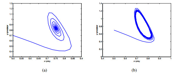
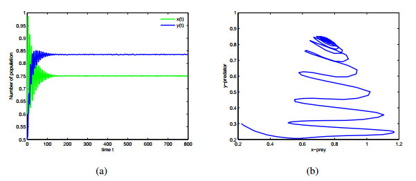
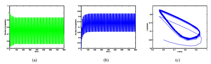
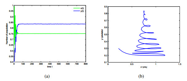
  • This article has been cited by:

    1. Saqib Ali, Jianqiang Li, Yan Pei, Muhammad Saqlain Aslam, Zeeshan Shaukat, Muhammad Azeem, An Effective and Improved CNN-ELM Classifier for Handwritten Digits Recognition and Classification, 2020, 12, 2073-8994, 1742, 10.3390/sym12101742
    2. Zhongze Wu, Chunmei He, Liwen Yang, Fangjun Kuang, Attentive evolutionary generative adversarial network, 2021, 51, 0924-669X, 1747, 10.1007/s10489-020-01917-8
    3. Jinghan Shang, Fei Shao, Jun Liu, Design of the Music Intelligent Management System Based on a Deep CNN, 2022, 2022, 1939-0122, 1, 10.1155/2022/1559726
    4. Xiufen Luo, Pan Zheng, Analysis the Innovation Path on Psychological Ideological with Political Teaching in Universities by Big Data in New Era, 2022, 2022, 1748-6718, 1, 10.1155/2022/4305886
    5. G. D. Praveenkumar, Dr. R. Nagaraj, Deep Convolutional Neural Network Based Extreme Learning Machine Image Classification, 2021, 2394-4099, 30, 10.32628/IJSRSET1218475
    6. Hui Deng, Zhibin Ou, Yichuan Deng, Multi-Angle Fusion-Based Safety Status Analysis of Construction Workers, 2021, 18, 1660-4601, 11815, 10.3390/ijerph182211815
    7. Songjian Dan, 2022, Chapter 7, 978-3-030-89507-5, 50, 10.1007/978-3-030-89508-2_7
    8. Li Lin, Wen Gan, Yuchen Li, 3D Simulation Design and Application of Traditional Hanfu Based on Internet of Things, 2022, 2022, 1607-887X, 1, 10.1155/2022/6977485
    9. Chunmei He, Lanqing Zheng, Taifeng Tan, Xianjun Fan, Zhengchun Ye, Manifold discrimination partial adversarial domain adaptation, 2022, 252, 09507051, 109320, 10.1016/j.knosys.2022.109320
    10. Lijun Zhou, Wei Liao, Dongyang Wang, Dong Wang, Guinan Zhang, Yi Cui, Junyi Cai, A High-Precision Diagnosis Method for Damp Status of OIP Bushing, 2021, 70, 0018-9456, 1, 10.1109/TIM.2020.3047194
    11. Ya'nan Wang, Sen Liu, Haijun Jia, Xintao Deng, Chunpu Li, Aiguo Wang, Cuiwei Yang, A two-step method for paroxysmal atrial fibrillation event detection based on machine learning, 2022, 19, 1551-0018, 9877, 10.3934/mbe.2022460
    12. Zhiping Song, 2022, Mathematical Modeling Method based on Neural Network and Computer Multi-Dimensional Space, 978-1-7281-8115-8, 1080, 10.1109/ICETCI55101.2022.9832088
    13. Shaojing Liu, Analysis on the literature communication path of new media integrating public mental health, 2022, 13, 1664-1078, 10.3389/fpsyg.2022.997558
    14. Haiyao Wang, Bolin Dai, Xiaolei Li, Naiwen Yu, Jingyang Wang, A Novel Hybrid Model of CNN-SA-NGU for Silver Closing Price Prediction, 2023, 11, 2227-9717, 862, 10.3390/pr11030862
    15. Subramanian. M, Md. Abul Ala Walid, Dr. Sarada Prasanna Mallick, Ravi Rastogi, Amit Chauhan, A. Vidya, 2023, Melanoma Skin Cancer Detection using a CNN-Regularized Extreme Learning Machine (RELM) based Model, 979-8-3503-4664-0, 1239, 10.1109/ICEARS56392.2023.10085489
    16. Yiyun Zhang, Sheng'an Zhou, 2022, Face Feature Extraction Algorithm Based on Wavelet Transform and CNN, 978-1-6654-9721-3, 111, 10.1109/ICITBS55627.2022.00032
    17. Shahad Altamimi, Qasem Abu Al-Haija, Maximizing intrusion detection efficiency for IoT networks using extreme learning machine, 2024, 4, 2730-7239, 10.1007/s43926-024-00060-x
    18. Lansa Ding, Xiaoyi Wei, Dezheng Wang, Congyan Chen, Construction of multi-features comprehensive indicator for machinery health state assessment, 2024, 35, 0957-0233, 066202, 10.1088/1361-6501/ad2bcb
    19. Qi Shi, Yanlei Li, Fan Zhang, Qianyun Ma, Jianfeng Sun, Yaqiong Liu, Jianlou Mu, Wenxiu Wang, Yiwei Tang, Whale optimization algorithm-based multi-task convolutional neural network for predicting quality traits of multi-variety pears using near-infrared spectroscopy, 2024, 215, 09255214, 113018, 10.1016/j.postharvbio.2024.113018
    20. Zhenhao Zhu, Qiushuang Zheng, Hongbing Liu, Jingyang Zhang, Tong Wu, Xianqiang Qu, Prediction Model for Pipeline Pitting Corrosion Based on Multiple Feature Selection and Residual Correction, 2024, 1671-9433, 10.1007/s11804-024-00468-5
    21. Zhicheng Liu, Long Zhao, Guanru Wen, Peng Yuan, Qiu Jin, A Monitoring Method for Transmission Tower Foots Displacement Based on Wind-Induced Vibration Response, 2023, 17, 1930-2991, 541, 10.32604/sdhm.2023.029760
    22. Manjula Prabakaran, Jesmin Zakaria, S Kannan, Santhiya P, Rajasekar P, M V Rathnamma, 2025, Enhancing Kidney Stone Detection in CT scans with Image Processing and the DCNN-RELM Model, 979-8-3315-0967-5, 1317, 10.1109/ICEARS64219.2025.10940943
  • Reader Comments
  • © 2019 the Author(s), licensee AIMS Press. This is an open access article distributed under the terms of the Creative Commons Attribution License (http://creativecommons.org/licenses/by/4.0)
通讯作者: 陈斌, bchen63@163.com
  • 1. 

    沈阳化工大学材料科学与工程学院 沈阳 110142

  1. 本站搜索
  2. 百度学术搜索
  3. 万方数据库搜索
  4. CNKI搜索

Metrics

Article views(5523) PDF downloads(912) Cited by(14)

Figures and Tables

Figures(9)

Other Articles By Authors

/

DownLoad:  Full-Size Img  PowerPoint
Return
Return

Catalog