Construction quality control of concrete structures in architectural engineering—A case in Shanghai, China

Francis Deng; Armin Mehdipour; Ali Soltani; Francis Deng; Armin Mehdipour; Ali Soltani

doi:10.3934/urs.2024013

Urban Resilience and Sustainability

2024, Volume 2, Issue 3: 256-271. doi: 10.3934/urs.2024013

Previous Article Next Article

Research article Special Issues

Construction quality control of concrete structures in architectural engineering—A case in Shanghai, China

1.
School of Art (Architecture), Nantong University, Nantong, Jiangsu, China
2.
School of Architecture and Civil Engineering, University of Adelaide, Adelaide, South Australia, Australia
3.
Healthy Communities, FHMRI, Bedford Park, Flinders University, South Australia, 5042, Australia

Received: 29 May 2024 Revised: 08 August 2024 Accepted: 20 August 2024 Published: 04 September 2024

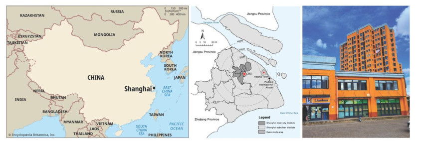
Architectural concrete provides diverse patterns, colors, and forms, offering extensive structural and aesthetic possibilities. In China, advanced techniques such as prefabricated and precast concrete structures are increasingly utilized, delivering benefits like faster construction, reduced resource use, and improved quality control. Recent studies in China have highlighted the environmental benefits and practical considerations of incorporating recycled materials and moderate-heat Portland cement into concrete, which offer promising sustainability advantages. This study, through a case analysis in China, explored the usability, durability, manufacturing costs, and economic implications of architectural concrete. It emphasizes the critical role of architectural concrete in modern structural engineering, financial planning, and design, aiming to reduce variability in strength and uniformity between concrete batches, ensure consistent material quality, and lower maintenance costs while accelerating production. Focusing on quality control in concrete construction in Heqing, Pudong, Shanghai, this research identified unique challenges and provided insights. In Shanghai's architectural context, continuous monitoring of concrete quality is essential for structural stability and durability. This study also addressed the resilience of concrete structures in saltwater and freeze-thaw conditions, underscoring the need to consider environmental factors in quality assurance. Laboratory experiments demonstrated that composite members and deep beams of steel and concrete exhibit notable deformation and shear resistance, highlighting the importance of meticulous material selection and structural design for effective quality control.
- architectural concrete,
- quality control,
- structural stability,
- sustainable construction,
- innovative design,
- Shanghai
Citation: Francis Deng, Armin Mehdipour, Ali Soltani. Construction quality control of concrete structures in architectural engineering—A case in Shanghai, China[J]. Urban Resilience and Sustainability, 2024, 2(3): 256-271. doi: 10.3934/urs.2024013

Related Papers:

Abstract

Architectural concrete provides diverse patterns, colors, and forms, offering extensive structural and aesthetic possibilities. In China, advanced techniques such as prefabricated and precast concrete structures are increasingly utilized, delivering benefits like faster construction, reduced resource use, and improved quality control. Recent studies in China have highlighted the environmental benefits and practical considerations of incorporating recycled materials and moderate-heat Portland cement into concrete, which offer promising sustainability advantages. This study, through a case analysis in China, explored the usability, durability, manufacturing costs, and economic implications of architectural concrete. It emphasizes the critical role of architectural concrete in modern structural engineering, financial planning, and design, aiming to reduce variability in strength and uniformity between concrete batches, ensure consistent material quality, and lower maintenance costs while accelerating production. Focusing on quality control in concrete construction in Heqing, Pudong, Shanghai, this research identified unique challenges and provided insights. In Shanghai's architectural context, continuous monitoring of concrete quality is essential for structural stability and durability. This study also addressed the resilience of concrete structures in saltwater and freeze-thaw conditions, underscoring the need to consider environmental factors in quality assurance. Laboratory experiments demonstrated that composite members and deep beams of steel and concrete exhibit notable deformation and shear resistance, highlighting the importance of meticulous material selection and structural design for effective quality control.

References

[1]	Mishra V, Sadhu A (2023) Towards the effect of climate change in structural loads of urban infrastructure: A review. Sustain Cities Soc 89: 104352. https://doi.org/10.1016/j.scs.2022.104352 doi: 10.1016/j.scs.2022.104352
[2]	Ghosn M, Frangopol DM, McAllister TP, et al. (2016) Reliability-based performance indicators for structural members. J Struct Eng 142: F4016002. https://doi.org/10.1061/(ASCE)ST.1943-541X.0001546
[3]	Alexander M, Beushausen H (2019) Durability, service life prediction, and modelling for reinforced concrete structures–review and critique. Cem Concr Res 122: 17–29. https://doi.org/10.1016/j.cemconres.2019.04.018 doi: 10.1016/j.cemconres.2019.04.018
[4]	Li Z, Zhou X, Ma H, et al. (2022) Advanced Concrete Technology, Hoboken: John Wiley & Sons.
[5]	Deng F, Hong Z (2013) Focus on sustainable bearing structures. Appl Mech Mater 405: 1182–1186. https://doi.org/10.4028/www.scientific.net/AMM.405-408.1182 doi: 10.4028/www.scientific.net/AMM.405-408.1182
[6]	Zhang S, Teizer J, Lee JK, et al. (2013) Building information modeling (BIM) and safety: Automatic safety checking of construction models and schedules. Autom Constr 29: 183–195. https://doi.org/10.1016/j.autcon.2012.05.006 doi: 10.1016/j.autcon.2012.05.006
[7]	Chang R, Zhang N, Gu Q (2023) A review on mechanical and structural performances of precast concrete buildings. Buildings 13: 1575. https://doi.org/10.3390/buildings13071575 doi: 10.3390/buildings13071575
[8]	Spasiano D, Marotta R, Malato S, et al. (2015) Solar photocatalysis: Materials, reactors, some commercial, and pre-industrialized applications. A comprehensive approach. Appl Catal B-environ 170: 90–123. https://doi.org/10.1016/j.apcatb.2014.12.050 doi: 10.1016/j.apcatb.2014.12.050
[9]	Al-Hasani LE, Park J, Perez G, et al. (2022) Quantifying concrete adiabatic temperature rise based on temperature-dependent isothermal calorimetry; modeling and validation. Mater Struct 55: 191. https://doi.org/10.1617/s11527-022-02023-6 doi: 10.1617/s11527-022-02023-6
[10]	Li C (2023) Economic Development of Communist China: An Appraisal of the First Five Years of Industrialization, London: Univ of California Press.
[11]	Genc O (2023) Identifying principal risk factors in Turkish construction sector according to their probability of occurrences: a relative importance index (RⅡ) and exploratory factor analysis (EFA) approach. Int J Proj Manag 23: 979–987. https://doi.org/10.1080/15623599.2021.1946901 doi: 10.1080/15623599.2021.1946901
[12]	Kibert CJ (2016) Sustainable Construction: Green Building Design and Delivery, Hoboken: John Wiley & Sons.
[13]	Mostafaei H, Badarloo B, Chamasemani NF, et al. (2023) Investigating the effects of concrete mix design on the environmental impacts of reinforced concrete structures. Buildings 13: 1313. https://doi.org/10.3390/buildings13051313 doi: 10.3390/buildings13051313
[14]	Han B, Zhang L, Ou J (2017) Smart and Multifunctional Concrete toward Sustainable Infrastructures, Singapore: Springer.
[15]	Yuan X, Moreu F, Hojati M (2021) Cost-effective inspection of rebar spacing and clearance using RGB-D sensors. Sustainability 13: 12509. https://doi.org/10.3390/su132212509 doi: 10.3390/su132212509
[16]	Yang Z, Tang M, Ji X, et al. (2018) Real-time strength prediction of different types of concrete based on BP neural network. NeuroQuantology 16: 650–656. https://doi.org/10.14704/nq.2018.16.6.1590 doi: 10.14704/nq.2018.16.6.1590
[17]	Gjørv OE (2011) Durability of concrete structures. Arab J Sci Eng 36: 151–172. https://doi.org/10.1007/s13369-010-0033-5 doi: 10.1007/s13369-010-0033-5
[18]	Lee HM, Lee HS, Min S, et al. (2018) Carbonation-induced corrosion initiation probability of rebars in concrete with/without finishing materials. Sustainability 10: 3814. https://doi.org/10.3390/su10103814 doi: 10.3390/su10103814
[19]	Chen J, Chen Y (2019) Research on corrosion detection and assessment method for hydraulic concrete structures. IOP Conf Ser: Mater Sci Eng 300: 052045. https://doi.org/10.1088/1755-1315/300/5/052045 doi: 10.1088/1755-1315/300/5/052045
[20]	Evstigneeva Y, Ibragimov R (2020) Construction technology of fixed formwork and quality control. IOP Conf Ser: Mater Sci Eng 890: 012131. https://doi.org/10.1088/1757-899X/890/1/012131 doi: 10.1088/1757-899X/890/1/012131
[21]	Belentsov YA, Egorov VV, Abu-Khasan MS, et al. (2022) Influence of the accuracy of strength control on the quality of the structures being erected. IOP Conf Ser: Mater Sci Eng 988: 052048. https://doi.org/10.1088/1755-1315/988/5/052048 doi: 10.1088/1755-1315/988/5/052048
[22]	Li J, Liu S, Liu A, et al. (2022) Knowledge graph construction for SOFL formal specifications. Int J Softw Eng Know 32: 605–644. https://doi.org/10.1142/S0218194022500279 doi: 10.1142/S0218194022500279
[23]	Dang Q, Miao R, Liang Y (2020) COVID-19 in Shang Hai: It is worth learning from the successful experience in preventing and controlling the overseas epidemic situation. medRxiv 2020: 20100164. https://doi.org/10.1101/2020.05.13.20100164 doi: 10.1101/2020.05.13.20100164
[24]	Wang SR, Wu XG, Yang JH, et al. (2020) Mechanical behavior of lightweight concrete structures subjected to 3D coupled static–dynamic loads. Acta Mech 231: 4497–4511.
[25]	Eller B, Movahedi Rad M, Fekete I, et al. (2023) Examination of concrete canvas under quasi-realistic loading by computed tomography. Infrastructures 8: 23. https://doi.org/10.3390/infrastructures8020023 doi: 10.3390/infrastructures8020023
[26]	Fayed S, Madenci E, Özkiliç YO, et al. (2023) Improving bond performance of ribbed steel bars embedded in recycled aggregate concrete using steel mesh fabric confinement. Constr Build Mater 369: 130452. https://doi.org/10.1016/j.conbuildmat.2023.130452 doi: 10.1016/j.conbuildmat.2023.130452
[27]	Le TT, Austin SA, Lim S, et al. (2012) Mix design and fresh properties for high-performance printing concrete. Mater Struct 45: 1221–1232. https://doi.org/10.1617/s11527-012-9828-z doi: 10.1617/s11527-012-9828-z
[28]	Su N, Miao B (2003) A new method for the mix design of medium strength flowing concrete with low cement content. Cem Concr Compos 25: 215–222. https://doi.org/10.1016/S0958-9465(02)00013-6 doi: 10.1016/S0958-9465(02)00013-6
[29]	Harris F, McCaffer R, Baldwin A, et al. (2021) Modern Construction Management, Hoboken: John Wiley & Sons.
[30]	Tay YWD, Qian Y, Tan MJ (2019) Printability region for 3D concrete printing using slump and slump flow test. Compos B Eng 174: 106968. https://doi.org/10.1016/j.compositesb.2019.106968 doi: 10.1016/j.compositesb.2019.106968
[31]	Voss G (2024) Systems Ultra: Making Sense of Technology in a Complex World, London: Verso Books.
[32]	Kinable J, Wauters T, Berghe GV (2014) The concrete delivery problem. Comput Oper Res 48: 53–68. https://doi.org/10.1016/j.cor.2014.02.008 doi: 10.1016/j.cor.2014.02.008
[33]	Kyriakides S, Corona E (2023) Mechanics of Offshore Pipelines: Volume I: Buckling and collapse, Houston: Gulf Professional Publishing.
[34]	Jahandari S, Tao Z, Chen Z, et al. (2023) Coal wastes: Handling, pollution, impacts, and utilization, In: The Coal Handbook, Elsevier, 97–163. https://doi.org/10.1016/B978-0-12-824327-5.00001-6
[35]	Sun W, Gao T, Zhao J, et al. (2023) Research on fracture behavior and reinforcement mechanism of fiber-reinforced locally layered backfill: Experiments and models. Constr Build Mater 366: 130186. https://doi.org/10.1016/j.conbuildmat.2022.130186 doi: 10.1016/j.conbuildmat.2022.130186
[36]	De Silva CW (2006) Vibration: Fundamentals and Practice, CRC press.
[37]	Scheffer C, Girdhar P (2004) Practical Machinery Vibration Analysis and Predictive Maintenance, Elsevier.
[38]	Weerapura V, Sugathadasa R, De Silva MM, et al. (2023) Feasibility of digital twins to manage the operational risks in the production of a ready-mix concrete plant. Buildings 13: 447. https://doi.org/10.3390/buildings13020447 doi: 10.3390/buildings13020447
[39]	Reyes W, Guzmán A (2011) Evaluation of the slenderness ratio in built-up cold-formed box sections. J Constr Steel Res 67: 929–935. https://doi.org/10.1016/j.jcsr.2011.02.003 doi: 10.1016/j.jcsr.2011.02.003
[40]	Li S, Li J (2017) Condition monitoring and diagnosis of power equipment: Review and prospective. High Volt 2: 82–91. https://doi.org/10.1049/hve.2017.0026 doi: 10.1049/hve.2017.0026
[41]	Aguilar E, Auer I, Brunet M, et al. (2003) Guidance on metadata and homogenization. Wmo Td 1186: 1–53.
[42]	Al-Barqawi M, Aqel R, Wayne M, et al. (2021) Polymer geogrids: A review of material, design and structure relationships. Materials 14: 4745. https://doi.org/10.3390/ma14164745 doi: 10.3390/ma14164745
[43]	Ellis EA, Springman SM (2001) Full-height piled bridge abutments constructed on soft clay. Geotechnique 51: 3–14. https://doi.org/10.1680/geot.2001.51.1.3 doi: 10.1680/geot.2001.51.1.3
[44]	Liu X, Wang J, Zhou X, et al. (2024) Response of long–short supporting piles due to deep excavation in soil–rock combined strata. Int J Geomech 24: 04023276. https://doi.org/10.1061/IJGNAI.GMENG-8587 doi: 10.1061/IJGNAI.GMENG-8587
[45]	Omrany H, Soebarto V, Sharifi E, et al. (2020) Application of life cycle energy assessment in residential buildings: A critical review of recent trends. Sustainability 12: 351. https://doi.org/10.3390/su12010351 doi: 10.3390/su12010351
[46]	Soltani A, Sharifi E (2017) Daily variation of urban heat island effect and its correlations to urban greenery: A case study of Adelaide. Front Archit Res 6: 529–538. https://doi.org/10.1016/j.foar.2017.08.001 doi: 10.1016/j.foar.2017.08.001
[47]	Soltani A, Sharifi E (2019) Understanding and analysing the urban heat island (UHI) effect in micro-scale. Int J Soc Ecol Sustain Dev (IJSESD) 10: 14–28. https://doi.org/10.4018/IJSESD.2019040102 doi: 10.4018/IJSESD.2019040102

Reader Comments

Your name:*

Email:*
© 2024 the Author(s), licensee AIMS Press. This is an open access article distributed under the terms of the Creative Commons Attribution License (http://creativecommons.org/licenses/by/4.0)