In recent years, opinion dynamics has received an increasing attention and various models have been introduced and evaluated mainly by simulation. In this study, we introduce a model inspired by the so-called "bounded confidence" approach where voters engaged in an electoral decision with two options are influenced by individuals sharing an opinion similar to their own. This model allows one to capture salient features of the evolution of opinions and results in final clusters of voters. We provide a detailed study of the model, including a complete taxonomy of the equilibrium points and an analysis of their stability. The model highlights that the final electoral outcome depends on the level of interaction in the society, besides the initial opinion of each individual, so that a strongly interconnected society can reverse the electoral outcome as compared to a society with looser exchange.
Citation: Sergei Yu. Pilyugin, M. C. Campi. Opinion formation in voting processes under bounded confidence[J]. Networks and Heterogeneous Media, 2019, 14(3): 617-632. doi: 10.3934/nhm.2019024
In recent years, opinion dynamics has received an increasing attention and various models have been introduced and evaluated mainly by simulation. In this study, we introduce a model inspired by the so-called "bounded confidence" approach where voters engaged in an electoral decision with two options are influenced by individuals sharing an opinion similar to their own. This model allows one to capture salient features of the evolution of opinions and results in final clusters of voters. We provide a detailed study of the model, including a complete taxonomy of the equilibrium points and an analysis of their stability. The model highlights that the final electoral outcome depends on the level of interaction in the society, besides the initial opinion of each individual, so that a strongly interconnected society can reverse the electoral outcome as compared to a society with looser exchange.

| [1] |
Cluster formation in opinion dynamics: A qualitative analysis. Z. Angew. Math. Phys. (2010) 61: 583-602. 
|
| [2] |
Asymptotic analysis of continuous opinion dynamics models under bounded confidence. Commun. Pure Appl. Anal. (2013) 12: 1487-1499.
|
| [3] |
Continuous and discontinuous opinion dynamics with bounded confidence. Nonlinear Anal. Real World Appl. (2012) 13: 1239-1251.
|
| [4] |
S. Chatterjee, Reaching a consensus: Some limit theorems, Proc. Int. Statist. Inst., 159–164. |
| [5] |
Toward consensus: Some convergence theorems on repeated averaging. J. Appl. Prob. (1977) 14: 89-97.
|
| [6] |
Approaching consensus can be delicate when positions harden. Stochastic Proc. and Appl. (1986) 22: 315-322.
|
| [7] | Mixing beliefs among interacting agents. Advances in Complex Systems (2000) 3: 87-98. |
| [8] |
Consensus formation under bounded confidence. Nonlinear Analysis (2001) 47: 4615-4621.
|
| [9] |
The Krause – Hegselmann consensus model with discrete opinions. Internat. J. Modern Phys. C (2004) 15: 1021-1029.
|
| [10] |
A formal theory of social power. Psychological Review (1956) 63: 181-194.
|
| [11] | Reaching a consensus. J. Amer. Statist. Assoc. (1974) 69: 118-121. |
| [12] |
F. Harary, A criterion for unanimity in French's theory of social power, in Studies in Social Power (ed. D. Cartwright), Institute for Social Research, Ann Arbor, 1959. |
| [13] |
The Hegselmann – Krause dynamics for equally spaced agents. J. Difference Equ. Appl. (2016) 22: 1621-1645.
|
| [14] |
R. Hegselmann and A. Flache, Understanding complex social dynamics: A plea for cellular automata based modelling, Journal of Artificial Societies and Social Simulation, 1 (1998). |
| [15] | Opinion dynamics and bounded confidence: Models, analysis and simulation. Journal of Artificial Societies and Social Simulation (2002) 5: 1-33. |
| [16] |
Opinion dynamics under the influence of radical groups, charismatic leaders, and other constant signals: A simple unifying model. Networks and Heterogeneous Media (2015) 10: 477-509.
|
| [17] |
Clustering and asymptotic behavior in opinion formation. J. Differential Equations (2014) 257: 4165-4187.
|
| [18] |
U. Krause, A discrete nonlinear and non - autonomous model of consensus formation, in Communications in Difference Equations (ed. S. Elaydi et al.), Gordon and Breach Publ., Amsterdam, 2000. |
| [19] |
U. Krause, Soziale dynamiken mit vielen interakteuren. eine problemskizze, in Modellierung und Simulation von Dynamiken mit vielen interagierenden Akteuren (eds. U. Krause and M. Stockler), Universitat Bremen, 1997. |
| [20] |
Compromise, consensus, and the iteration of means. Elem. Math. (2009) 64: 1-8.
|
| [21] |
U. Krause, Positive Dynamical Systems in Discrete Time. Theory, Models, and Applications, De Gruyter, Berlin, 2015. |
| [22] |
On the Hegselmann – Krause conjecture in opinion dynamics. Journal of Difference Equations and Applications (2011) 17: 859-876.
|
| [23] |
Social consensus and rational agnoiology. Synthese (1975) 31: 141-160.
|
| [24] |
K. Lehrer and C. Wagner, Rational Consensus in Science and Society, D. Reidel Publ. Co., Dordrecht-Boston, Mass., 1981. |
| [25] |
A stabilization theorem for dynamics of continuous opinions. Physica A (2005) 355: 217-223.
|
| [26] |
Continuous opinion dynamics under bounded confidence: A survey. International Journal of Modern Physics C (2007) 18: 1819-1838.
|
| [27] |
W. Ren and Y. Cao, Distributed Coordination of Multi-agent Networks. Emergent Problems, Models, and Issues, Springer, 2011. |
| [28] |
Consensus through respect: A model of rational group decision-making. Philosophical Studies (1978) 34: 335-349.
|
| [29] |
The Hegselmann – Krause dynamics for the continuous-agent model and a regular opinion function do not always lead to consensus. IEEE Trans. Automat. Control (2015) 60: 2416-2421.
|
| [30] |
G. Weisbuch, G. Deffuant and G. Nadal, Interacting agents and continuous opinion dynamics, in Heterogenous Agents, Interactions and Economic Performance (eds. R. Cowan and N. Jonard), Lecture Notes in Economics and Mathematical Systems, 521, Springer, Berlin, 2003. |
| [31] |
On the control through leadership of the Hegselmann – Krause opinion formation model. Mathematical Models and Methods in Applied Sciences (2015) 25: 565-585.
|


Figures(5)
Sergei Yu. Pilyugin, M. C. Campi. Opinion formation in voting processes under bounded confidence[J]. Networks and Heterogeneous Media, 2019, 14(3): 617-632. doi: 10.3934/nhm.2019024

Initial distribution of opinions for the first example
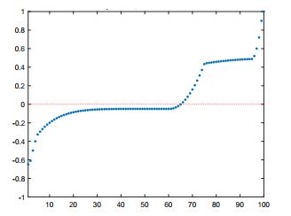
Opinions' evolution for first example at steps
Initial distribution of opinions for the second example
Opinions' evolution for second example at steps
Opinions' evolution for second example at steps


 DownLoad: