In vitro anti-trypanosomal activity of crude extract and fractions of Trichoscypha acuminata stem bark, Spathodea campanulata flowers, and Ficus elastica lianas on Trypanosoma brucei brucei

Jean Emmanuel Mbosso Teinkela; Philippe Belle Ebanda Kedi; Jean Baptiste Hzounda Fokou; Michelle Isaacs; Lisette Pulchérie Yoyo Ngando; Gaelle Wea Tchepnou; Hassan Oumarou; Xavier Siwe Noundou; Jean Emmanuel Mbosso Teinkela; Philippe Belle Ebanda Kedi; Jean Baptiste Hzounda Fokou; Michelle Isaacs; Lisette Pulchérie Yoyo Ngando; Gaelle Wea Tchepnou; Hassan Oumarou; Xavier Siwe Noundou

doi:10.3934/molsci.2024005

AIMS Molecular Science

2024, Volume 11, Issue 1: 63-71. doi: 10.3934/molsci.2024005

Previous Article Next Article

Research article Topical Sections

In vitro anti-trypanosomal activity of crude extract and fractions of Trichoscypha acuminata stem bark, Spathodea campanulata flowers, and Ficus elastica lianas on Trypanosoma brucei brucei

1.
Department of Biological Sciences, Faculty of Medicine and Pharmaceutical Sciences, University of Douala, P.O. Box. 2701 Douala, Cameroon
2.
Department of Pharmaceutical Sciences, Faculty of Medicine and Pharmaceutical Sciences, University of Douala, P.O. Box. 2701 Douala, Cameroon
3.
Faculty of Pharmacy, Rhodes University, Grahamstown, 6140, South Africa
4.
Department of Pharmaceutical Sciences, School of Pharmacy, Sefako Makgatho Health Sciences University, P.O. Box 218 MEDUNSA, Pretoria 0204, South Africa

Received: 29 September 2023 Revised: 23 January 2024 Accepted: 23 January 2024 Published: 06 February 2024

The low therapeutic index of available trypanocidal drugs and the increasing emergence of resistant Trypanosoma parasites indicate the urgent need to develop new strategies for trypanosomiasis control. One such strategy is the screening of medicinal plants as sources of new lead compounds. Trypanosoma brucei brucei is a sub-species only infecting animals and thus largely used to screen anti-trypanosomal potential of various substances. Therefore, the present study investigates the anti-trypanosomal activity of crude extract, hexane, dichloromethane, ethyl acetate, and aqueous fractions of Spathodea campanulata P. Beauv. flowers, Trichoscypha acuminata Engl. stem bark, and Ficus elastica Roxb. Ex Hornem lianas using the Alamar Blue assay. Overall results showed that the crude extract of T. acuminata, S. campanulate, and F. elastica did not significantly reduce the viability of Trypanosoma brucei brucei at the tested concentration of 25 µg/mL. However, the hexane and dichloromethane fractions of T. acuminata and the hexane fraction of F. elastica exhibited viability percentages of 23.2 ± 10.5, 18.2 ± 9.7, and 20.1 ± 13.1% with IC₅₀ values of 5.5, 5.0, and 17.5 µg/mL, respectively. Further research to identify compounds responsible for the observed activity and their mechanisms of action towards new leads in parasitical drug discovery is needed.
- Spathodea campanulata,
- Ficus elastica,
- Trichoscypha acuminata,
- anti-trypanosomal activity,
- Trypanosoma brucei brucei
Citation: Jean Emmanuel Mbosso Teinkela, Philippe Belle Ebanda Kedi, Jean Baptiste Hzounda Fokou, Michelle Isaacs, Lisette Pulchérie Yoyo Ngando, Gaelle Wea Tchepnou, Hassan Oumarou, Xavier Siwe Noundou. In vitro anti-trypanosomal activity of crude extract and fractions of Trichoscypha acuminata stem bark, Spathodea campanulata flowers, and Ficus elastica lianas on Trypanosoma brucei brucei[J]. AIMS Molecular Science, 2024, 11(1): 63-71. doi: 10.3934/molsci.2024005

Related Papers:

Abstract

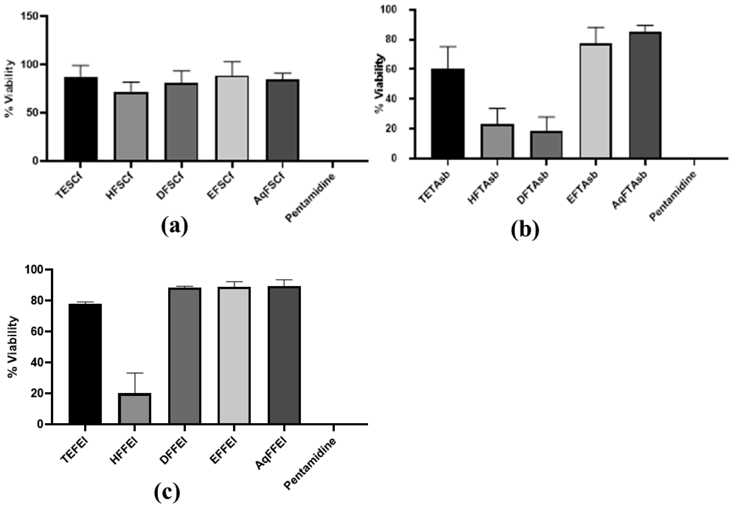
The low therapeutic index of available trypanocidal drugs and the increasing emergence of resistant Trypanosoma parasites indicate the urgent need to develop new strategies for trypanosomiasis control. One such strategy is the screening of medicinal plants as sources of new lead compounds. Trypanosoma brucei brucei is a sub-species only infecting animals and thus largely used to screen anti-trypanosomal potential of various substances. Therefore, the present study investigates the anti-trypanosomal activity of crude extract, hexane, dichloromethane, ethyl acetate, and aqueous fractions of Spathodea campanulata P. Beauv. flowers, Trichoscypha acuminata Engl. stem bark, and Ficus elastica Roxb. Ex Hornem lianas using the Alamar Blue assay. Overall results showed that the crude extract of T. acuminata, S. campanulate, and F. elastica did not significantly reduce the viability of Trypanosoma brucei brucei at the tested concentration of 25 µg/mL. However, the hexane and dichloromethane fractions of T. acuminata and the hexane fraction of F. elastica exhibited viability percentages of 23.2 ± 10.5, 18.2 ± 9.7, and 20.1 ± 13.1% with IC₅₀ values of 5.5, 5.0, and 17.5 µg/mL, respectively. Further research to identify compounds responsible for the observed activity and their mechanisms of action towards new leads in parasitical drug discovery is needed.

Acknowledgments

We would like to thank the Department of Biochemistry and Microbiology, Rhodes University, Grahamstown, South Africa for the anti-trypanosomal tests.

Conflict of interest

The authors declare no conflict of interest in this manuscript.

References

[1]	Oethinger MD, Campbell SM (2009) Infection and host response. Molecular pathology.Academic Press 42-61. https://doi.org/10.1016/B978-0-12-374419-7.00003-2
[2]	Richards S, Morrison LJ, Torr SJ, et al. (2021) Pharma to farmer: Field challenges of optimizing trypanocide use in African animal trypanosomiasis. Trends Parasitol 37: 831-843. https://doi.org/10.1016/j.pt.2021.04.007
[3]	Giordani F, Paape D, Vincent IM, et al. (2020) Veterinary trypanocidal benzoxaboroles are peptidase-activated prodrugs. PLoS Pathog 16: e1008932. https://doi.org/10.1371/journal.ppat.1008932
[4]	Crump RE, Huang CI, Knock ES, et al. (2021) Quantifying epidemiological drivers of gambiense human African trypanosomiasis across the Democratic Republic of Congo. PLoS Comput Biol 17: e1008532. https://doi.org/10.1371/journal.pcbi.1008532
[5]	Barrett MP, Boykin DW, Brun R, et al. (2007) Human African trypanosomiasis: Pharmacological re-engagement with a neglected disease. Br J Pharmacol 152: 1155-1171. https://doi.org/10.1038/sj.bjp.0707354
[6]	Remme JHF, Blas E, Chitsulo L, et al. (2002) Strategic emphases for tropical diseases research: A TDR perspective. Trends Microbiol 10: 435-440. https://doi.org/10.1016/S0966-842X(02)02431-9
[7]	Hosseinzadeh S, Jafarikukhdan A, Hosseini A, et al. (2015) The application of medicinal plants in traditional and modern medicine: A review of Thymus vulgaris. Int J Clin Med 6: 635-642. https://doi.org/10.4236/ijcm.2015.69084
[8]	Teinkela JEM, Noundou XS, Nguemfo EL, et al. (2018) Biological activities of plant extracts from Ficus elastica and Selaginella vogelli: An antimalarial, antitrypanosomal and cytotoxity evaluation. Saudi J Biol Sci 25: 117-122. https://doi.org/10.1016/j.sjbs.2017.07.002
[9]	Fouokeng Y, Feumo FHM, Mbosso TJE, et al. (2019) In vitro antimalarial, antitrypanosomal and HIV-1 integrase inhibitory activities of two Cameroonian medicinal plants: Antrocaryon klaineanum (Anacardiaceae) and Diospyros conocarpa (Ebenaceae). S Afr J Bot 122: 510-517. https://doi.org/10.1016/j.sajb.2018.10.008
[10]	Teinkela JEM, Noundou XS, Fannang SV, et al. (2019) Terminaliamide, a new ceramide and other phytoconstituents from the roots of Terminalia mantaly H. Perrier and their biological activities. Nat Prod Res 35: 1313-1322. https://doi.org/10.1080/14786419.2019.1647425
[11]	Teinkela JEM, Noundou XS, Mimba JEZ, et al. (2020) Compounds isolation and biological activities of Piptadeniastrum africanum (hook.f.) Brennan roots. J Ethnopharmacol 255: 112716. https://doi.org/10.1016/j.jep.2020.112716
[12]	Teinkela JEM, Yoyo NLP, Bamal HD, et al. (2023) Evaluation of in vitro antiplasmodial, anti-inflammatory activities and in vivo oral acute toxicity of Trichoscypha acuminata Engl. (Anacardiaceae) stem bark. Nat J Pharma Sci 3: 107-114.
[13]	Teinkela JEM, Oumarou H, Noundou XS, et al. (2023) Evaluation of in vitro antiplasmodial, antiproliferative activities, and in vivo oral acute toxicity of Spathodea campanulata flowers. Sci Afr 21: e01871. https://doi.org/10.1016/j.sciaf.2023.e01871
[14]	Teinkela JEM, Tchepnou GW, Ngo NC, et al. (2023) Antiproliferative, antimicrobial, antiplasmodial, and oral acute toxicity of Ficus elastica Roxb. Ex Hornem lianas. Invest Med Chem Pharmacol 6: 77. https://doi.org/10.31183/imcp.2023.00077
[15]	Ngozi NJ, Agbo M (2011) Antitrypanosomal effects of methanolic extract of Nauclea diderrichii (Merr) and Spathodea campaunlata stem bark. J Pharm Allied Sci 7: 1219-1227. https://doi.org/10.4314/jophas.v7i5.63466
[16]	Teinkela JEM, Noundou XS, Nguemfo EL, et al. (2018) Biological activities of plant extracts from Ficus elastica and Selaginella vogelli: An antimalarial, antitrypanosomal and cytotoxity evaluation. Saudi J Biol Sci 25: 117-122. https://doi.org/10.1016/j.sjbs.2017.07.002
[17]	Bidié AP, Yapo FA, Yéo D, et al. (2010) Effet de Mitragyna ciliata (MYTA) sur le système cardiovasculaire de rat. Phytothérapie 8: 3-8. https://doi.org/10.1007/s10298-009-0519-z
[18]	Darrella OT, Hulushea ST, Mtshare TE, et al. (2018) Synthesis, antiplasmodial and antitrypanosomal evaluation of a series of novel 2-oxoquinoline-based thiosemicarbazone derivatives. S Afr J Chem 71: 174-181. https://doi.org/10.17159/0379-4350/2018/v71a23
[19]	The tropical plants databaseUseful tropical plants: Trichoscypha acuminata (2014). Available from: https://tropical.theferns.info/viewtropical.php?id=Trichoscypha+acuminata
[20]	Burkill HM The useful plants of West Tropical Africa (1985).
[21]	Consoli RA, Mendes NM, Pereira JP, et al. (1988) Effect of several extracts derived from plants on the survival of larvae of Aedes fluviatilis (Lutz) (Diptera: Culicidae) in the laboratory. Mem Inst Oswaldo Cruz 83: 87-93. https://doi.org/10.1590/s0074-02761988000100012
[22]	Gopal KP (2021) Spathodea campanulata P. Beauv. —A review of its ethnomedicinal, phytochemical, and pharmacological profile. J Appl Pharm Sci 11. https://doi.org/10.7324/JAPS.2021.1101202
[23]	Mpondo ME, Vandi D, Ngouondjou FT, et al. (2017) Contribution des populations des villages ducentre Cameroun aux traitements traditionnels des affections des voies respiratoires (In French). J Anim Plant Sci 32: 5223-5242.
[24]	Ochwang'I DO, Kimwele CN, Oduma JA, et al. (2014) Medicinal plants used in treatment and management of cancer in Kakamega County, Kenya. J Ethnopharmacol 151: 1040-1055. https://doi.org/10.1016/j.jep.2013.11.051
[25]	Rolland KG, Rostand OM, Dieudonne SK, et al. (2017) Enquête ethnopharmacologique des plantes antipaludiques dans le département d'Agboville, sud-est de la Cote d'Ivoire (In French). J Applied Biosci 109: 10618-10629. https://doi.org/10.4314/jab.v109i1.6
[26]	Bystrická J, Vollmannová A, Kupecsek A, et al. (2011) Bioactive compounds in different parts of various buckwheat (Fagopyrum esculentum Moench.) cultivars. Cereal Res Commun 39: 436-444. https://doi.org/10.1556/CRC.39.2011.3.13
[27]	Hoet S, Opperdoes F, Brun R, et al. (2004) Natural products active against African trypanosomes: A step towards new drugs. Nat Prod Rep 21: 353-364. https://doi.org/10.1039/b311021b
[28]	Sanderson L, Dogruel M, Rodgers J, et al. (2009) Pentamidine movement across the murine blood-brain and blood-cerebrospinal fluid barriers: effect of trypanosome infection, combination therapy, P-glycoprotein, and multidrug resistance-associated protein. J Pharmacol Exp Ther 329: 967-977. https://doi.org/10.1124/jpet.108.149872

Reader Comments

Your name:*

Email:*
© 2024 the Author(s), licensee AIMS Press. This is an open access article distributed under the terms of the Creative Commons Attribution License (http://creativecommons.org/licenses/by/4.0)