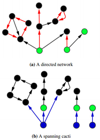
The control of complex networks has been studied extensively in the last decade, with different control models been introduced. In this paper, we propose a new network control framework, called local controllability. Local controllability extends the entire network control onto a local scale, and it concerns about the minimum number of inputs required to control a subset of nodes in a directed network. We develop a mathematical formulation for local controllability as an optimization problem and show that it can be solved by a cubic-time algorithm. Moreover, applications to both real networks and model networks are presented and results of these numerical studies are then discussed.
Citation: Chang Luo. Local controllability of complex networks[J]. Mathematical Modelling and Control, 2021, 1(2): 121-133. doi: 10.3934/mmc.2021010
The control of complex networks has been studied extensively in the last decade, with different control models been introduced. In this paper, we propose a new network control framework, called local controllability. Local controllability extends the entire network control onto a local scale, and it concerns about the minimum number of inputs required to control a subset of nodes in a directed network. We develop a mathematical formulation for local controllability as an optimization problem and show that it can be solved by a cubic-time algorithm. Moreover, applications to both real networks and model networks are presented and results of these numerical studies are then discussed.

| [1] | S. Boccaletti, V. Latora, Y. Moreno, M. Chavez, D. Hwang, Complex networks: structure and dynamics, Physics Reports, 424 (2006), 175–308. |
| [2] | M. Newman, The structure and function of complex networks, SIAM Rev., 45 (2003), 167–256. |
| [3] | A. Clauset, M. Newman, C. Moore, Finding community structure in very large networks, Phys. Rev. E, 70 (2004), 066111. |
| [4] | L. Freeman, Centrality in social networks conceptual clarification, Social Networks, 1 (1979), 215–239. |
| [5] | R. Milo, S. Shen-Orr, Kashtan, D. Chklovskii, U. Alon, Network motifs: simple building blocks of complex networks, Science, 298 (2002), 824–827. |
| [6] | A. L. Barabási, R. Albert, Emergence of scaling in random networks, Science, 286 (1999), 509–512. |
| [7] | D. Watts, S. Strogatz, Collective dynamics of 'small-world' networks, Nature, 393 (1998), 440–442. |
| [8] | R. Pastor-Satorras, A. Vespignani, Epidemic spreading in scale-free networks, Phys. Rev. Lett., 86 (2001), 3200–3203. |
| [9] | P. Oikonomou, P. Cluzel, Effects of topology on network evolution, Nat. Phys., 2 (2006), 532–536. |
| [10] | D. Callaway, M. Newman, S. Strogatz, D. Watts, Network robustness and fragility: percolation on random graphs, Phys. Rev. Lett., 85 (2000), 5468–5471. |
| [11] | F. Sorrentino, M. Bernardo, F. Garofalo, G. Chen, Controllability of complex networks via pinning, Phys. Rev. E, 75 (2007), 046103. |
| [12] | D. Luenberger, Introduction to Dynamical Systems: Theory, Models and Applications, 1979. |
| [13] | Y. Liu, J. Slotine, A. Barabási, Controllability of complex networks, Nature, 473 (2011), 167–173. |
| [14] | T. Nepusz, T. Vicsek, Controlling edge dynamics in complex networks, Nat. Phys., 8 (2012), 568–573. |
| [15] | Z. Yuan, C. Zhao, Z. Di, W. Wang, Y. Lai, Exact controllability of complex networks, Nat. Commun., 4 (2013), 1–9. |
| [16] | S. Hosoe, Determination of generic dimensions of controllable subspaces and its application, IEEE T. Automat. Contr., 25 (1980), 1192–1196. |
| [17] | Y. Liu, J. Slotine, A. Barabási, Control centrality and hierarchical structure in complex networks, PLos One, 7 (2012), e44459. |
| [18] | J. Gao, Y. Liu, R. D'Souza, A. Barabási, Target control of complex networks, Nat. Commun., 5 (2014), 1–8. |
| [19] | Y. Liu, A. Barabási, Control principles of complex systems, Rev. Mod. Phys., 88 (2016), 035006. |
| [20] | R. Kalman, Mathematical description of linear dynamical systems, J. Soc. Indus. Appl. Math. Ser. A, 1 (1963), 152–192. |
| [21] | C. Lin, Structural controllability, IEEE T. Automat. Contr., 19 (1974), 201–208. |
| [22] | K. Glover, L. Silverman, Characterization of structural controllability, IEEE T. Automat. Contr., 21 (1976), 534–537. |
| [23] | R. Shields, J. Pearson, Structural controllability of multi-input linear systems, IEEE T. Automat. Contr., 21 (1976), 203–212. |
| [24] | J. Dion, C. Commault, J. van der Woude, Generic properties and control of linear structured systems: a survey, Automatica, 39 (2003), 1125–1144. |
| [25] | H. Mayeda, On structural controllability theorem, IEEE T. Automat. Contr., 26 (1981), 795–798. |
| [26] | N. Ahn, Spanning Cacti for Structurally Controllable Networks, master thesis, National University of Singapore, 2012. |
| [27] | J. Hopcroft, R. Karp, An $n^{5/2}$ algorithm for maximum matchings in bipartite graphs, SIAM J. Comput., 2 (1973), 225–231. |
| [28] | P. Csermely, T. Korcsmaros, H. Kiss, G. London, R. Nussinov, Structure and dynamics of molecular networks: a novel paradigm of drug discovery, a comprehensive review, Pharmacology and Therapeutics, 138 (2013), 333–408. |
| [29] | H. Kuhn, The Hungarian method for the assignment problem, Naval Research Logistics Quarterly, 2 (1955), 83–97. |
| [30] | S. Oh, J. Harris, et al, A mesoscale connectome of the mouse brain, Nature, 508 (2014), 207–214. |
| [31] | M. Kirkcaldie, The Mouse Nervous System, (2012), 52–111. |
| [32] | L. Puelles, M. Martinez-De-La-Torre, J. Ferran, C. Watson, The Mouse Nervous System, (2012), 313–336. |
| [33] | P. Erdős, A. Rényi, On the evolution of random graphs, Publications of the Mathematical Institute of the Hungarian Academy of Science, 5 (1960), 17–61. |
| [34] | K. Goh, B. Kahng, D. Kim, Universal behavior of load distribution in scale-free networks, Phys. Rev. Lett., 87, (2001), 278701. |


Figures(6) / Tables(2)
Chang Luo. Local controllability of complex networks[J]. Mathematical Modelling and Control, 2021, 1(2): 121-133. doi: 10.3934/mmc.2021010


 DownLoad: