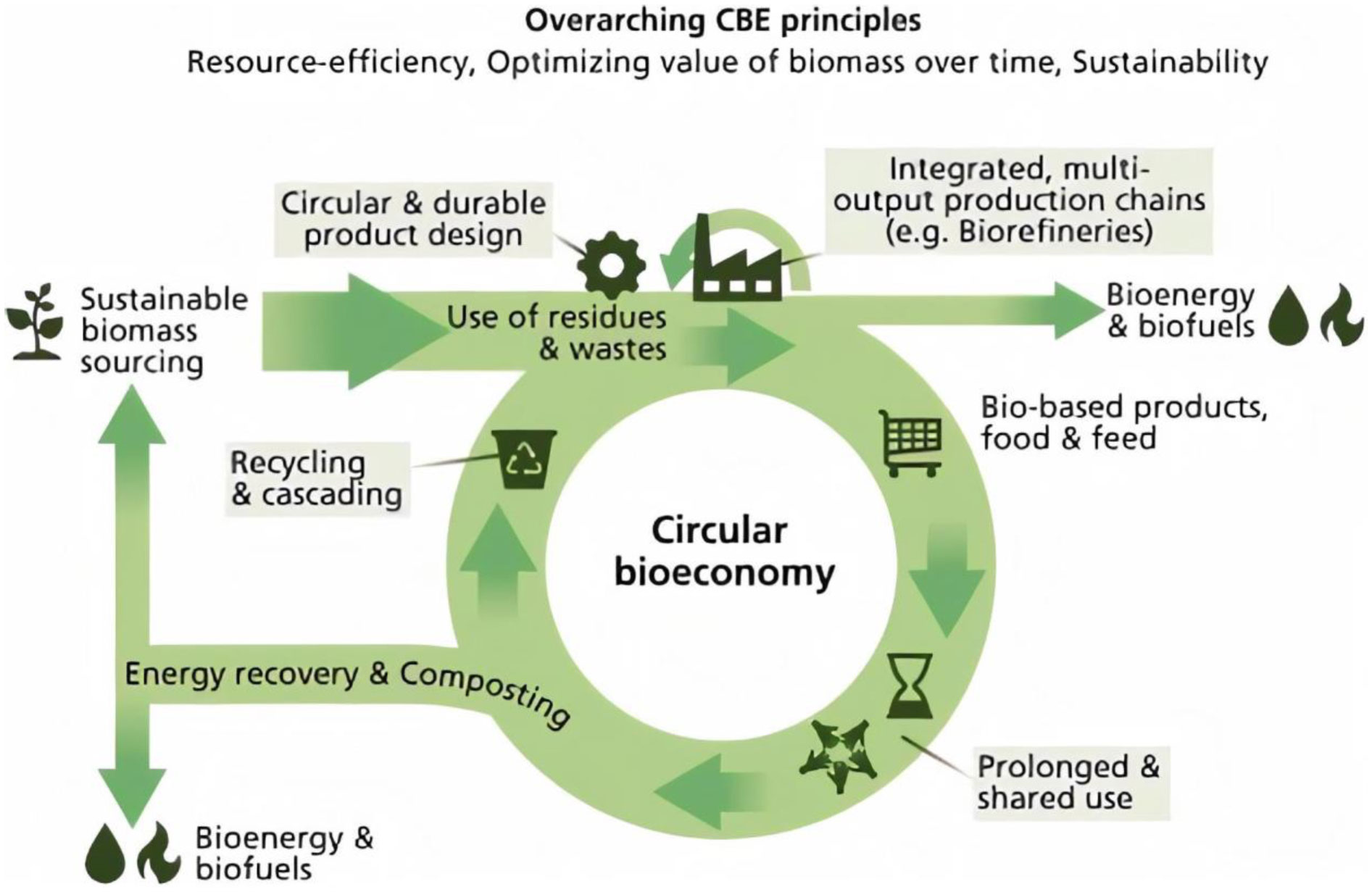
The circular bioeconomy has undoubtedly gained global momentum during the last few years. The bioeconomy envisions “3R”, the goal of 3R (Reduce, Recycle, Reuse) is to implement in circular economy preventing excessive and unnecessary wastes. The circular bioeconomy emphasizes the best use of all sorts of available bioresources through the reduction of generated wastes during product formation, recycling of generated wastes, and reuse of valuable by-products and residues. Biotechnology could be useful in utilizing the resources to the optimum and therefore the role of biological agents and bioprocesses is of prime importance. In this review, we highlight the paramount importance of beneficial strains of microorganisms, macro, and microalgae in the bioeconomy. Microorganisms are universally recognized for the notable production of a vast array of secondary metabolites and other functionalities with possible use in various sectors. The application of potential strains in industries and modern agriculture practices could progressively improve the effective yield of food and feed, including fertilization of arid soils, bioconversion of by-products from industrial processes, and agriculture wastes. The valuable properties of specifically selected biological agents typically make them suitable candidates for their efficient contribution to circular bioeconomy without hampering the environment.
Citation: Divakar Dahiya, Hemant Sharma, Arun Kumar Rai, Poonam Singh Nigam. Application of biological systems and processes employing microbes and algae to Reduce, Recycle, Reuse (3Rs) for the sustainability of circular bioeconomy[J]. AIMS Microbiology, 2022, 8(1): 83-102. doi: 10.3934/microbiol.2022008
The circular bioeconomy has undoubtedly gained global momentum during the last few years. The bioeconomy envisions “3R”, the goal of 3R (Reduce, Recycle, Reuse) is to implement in circular economy preventing excessive and unnecessary wastes. The circular bioeconomy emphasizes the best use of all sorts of available bioresources through the reduction of generated wastes during product formation, recycling of generated wastes, and reuse of valuable by-products and residues. Biotechnology could be useful in utilizing the resources to the optimum and therefore the role of biological agents and bioprocesses is of prime importance. In this review, we highlight the paramount importance of beneficial strains of microorganisms, macro, and microalgae in the bioeconomy. Microorganisms are universally recognized for the notable production of a vast array of secondary metabolites and other functionalities with possible use in various sectors. The application of potential strains in industries and modern agriculture practices could progressively improve the effective yield of food and feed, including fertilization of arid soils, bioconversion of by-products from industrial processes, and agriculture wastes. The valuable properties of specifically selected biological agents typically make them suitable candidates for their efficient contribution to circular bioeconomy without hampering the environment.

| [1] |
Cramer JM (2020) Practice-based model for implementing circular economy: The case of the Amsterdam Metropolitan Area. J Clean Prod 255: 120255. https://doi.org/10.1016/j.jclepro.2020.120255 
|
| [2] | The Ellen MacArthur FoundationEconomy global commitment (2021). Available from: https://ellenmacarthurfoundation.org/global-commitment/overview |
| [3] |
Buchmann-Duck J, Beazley KF (2020) An urgent call for circular economy advocates to acknowledge its limitations in conserving biodiversity. Sci Total Environ 727: 138602. https://doi.org/10.1016/j.scitotenv.2020.138602
|
| [4] |
Michelini G, Moraes RN, Cunha RN, et al. (2017) From linear to circular economy: PSS conducting the transition. Procedia CIRP 64: 2-6. https://doi.org/10.1016/j.procir.2017.03.012
|
| [5] |
Didenko NI, Klochkov YS, Skripnuk DF (2018) Ecological criteria for comparing linear and circular economies. Resources 7: 48. https://doi.org/10.3390/resources7030048
|
| [6] |
Clark JH, Farmer TJ, Herrero-Davila L, et al. (2016) Circular economy design considerations for research and process development in the chemical sciences. Green Chem 18: 3914-3934. https://doi.org/10.1039/C6GC00501B
|
| [7] |
Geissdoerfer M, Morioka SN, de Carvalho MM, et al. (2018) Business models and supply chains for the circular economy. J Clean Prod 190: 712-721. https://doi.org/10.1016/j.jclepro.2018.04.159
|
| [8] |
Cullen JM (2017) Circular economy: Theoretical benchmark or perpetual motion machine?. J Ind Ecol 21: 483-486. https://doi.org/10.1111/jiec.12599
|
| [9] |
Sherwood J (2020) The significance of biomass in a circular economy. Bioresour Technol 300. https://doi.org/10.1016/j.biortech.2020.122755
|
| [10] |
Falcone PM, González García S, Imbert E, et al. (2019) Transitioning towards the bio-economy: Assessing the social dimension through a stakeholder lens. Corp Soc Responsib Environ Manag 26: 1135-1153. https://doi.org/10.1002/csr.1791
|
| [11] |
Sanz-Hernández A, Esteban E, Garrido P (2019) Transition to a bioeconomy: Perspectives from social sciences. J Clean Prod 224: 107-119. https://doi.org/10.1016/j.jclepro.2019.03.168
|
| [12] |
Woźniak E, Tyczewska A, Twardowski T (2021) Bioeconomy development factors in the European Union and Poland. N Biotechnol 60: 2-8. https://doi.org/10.1016/j.nbt.2020.07.004
|
| [13] | Ronzon T, Iost S, Philippidis G (2022) Has the European Union entered a bioeconomy transition? Combining an output-based approach with a shift-share analysis. Env Dev Sustain . https://doi.org/10.1007/s10668-021-01780-8 |
| [14] |
Bugge MM, Hansen T, Klitkou A (2016) What is the bioeconomy? A review of the literature. Sustain 8: 691. https://doi.org/10.3390/su8070691
|
| [15] |
Carus M, Dammer L (2018) The circular bioeconomy-concepts, opportunities, and limitations. Ind Biotechnol 14: 83-91. https://doi.org/10.1089/ind.2018.29121.mca
|
| [16] |
Salvador R, Puglieri FN, Halog A, et al. (2021) Key aspects for designing business models for a circular bioeconomy. J Clean Prod 278: 124341. https://doi.org/10.1016/j.jclepro.2020.124341
|
| [17] |
Klitkou A, Fevolden AM, Capasso M From waste to value: Valorisation pathways for organic waste streams in circular bioeconomies, routledge (2019). https://doi.org/10.4324/9780429460289
|
| [18] |
Salvador R, Barros MV, Luz LM da, et al. (2020) Circular business models: Current aspects that influence implementation and unaddressed subjects. J Clean Prod 250: 119555. https://doi.org/10.1016/j.jclepro.2019.119555
|
| [19] |
Robert N, Giuntoli J, Araujo R, et al. (2020) Development of a bioeconomy monitoring framework for the European Union: An integrative and collaborative approach. N Biotechnol 59: 10-19. https://doi.org/10.1016/j.nbt.2020.06.001
|
| [20] | Stegmann P, Londo M, Junginger M (2020) The circular bioeconomy: Its elements and role in European bioeconomy clusters. Resour Conserv Recycl X 6: 100029. https://doi.org/10.1016/j.rcrx.2019.100029 |
| [21] |
Mikielewicz D, Dąbrowski P, Bochniak R, et al. (2020) Current status, barriers and development perspectives for circular bioeconomy in polish South Baltic Area. Sustainability 12: 9155. https://doi.org/10.3390/su12219155
|
| [22] |
Abbas F, Hammad HM, Anwar F, et al. (2021) Transforming a valuable bioresource to biochar, its environmental importance, and potential applications in boosting circular bioeconomy while promoting sustainable agriculture. Sustainability 13: 2599. https://doi.org/10.3390/su13052599
|
| [23] | Valix M (2017) Bioleaching of electronic waste: Milestones and challenges. Curr Dev Biotechnol Bioeng 7: 407-442. https://doi.org/10.1016/B978-0-444-63664-5.00018-6 |
| [24] |
Baniasadi M, Graves JE, Ray DA, et al. (2021) Closed-loop recycling of copper from waste printed circuit boards using bioleaching and electrowinning processes. Waste and Biomass Valorization 12: 3125-3136. https://doi.org/10.1007/s12649-020-01128-9
|
| [25] |
Nithya R, Sivasankari C, Thirunavukkarasu A (2021) Electronic waste generation, regulation and metal recovery: a review. Environ Chem Lett 19: 1347-1368. https://doi.org/10.1007/s10311-020-01111-9
|
| [26] |
Ilyas S, Srivastava RR, Kim H, et al. (2021) Circular bioeconomy and environmental benignness through microbial recycling of e-waste: A case study on copper and gold restoration. Waste Manag 121: 175-185. https://doi.org/10.1016/j.wasman.2020.12.013
|
| [27] |
Karan H, Funk C, Grabert M, et al. (2019) Green bioplastics as part of a circular bioeconomy. Trends Plant Sci 24: 237-249. https://doi.org/10.1016/j.tplants.2018.11.010
|
| [28] |
Meixner K, Kovalcik A, Sykacek E, et al. (2018) Cyanobacteria biorefinery-production of poly(3-hydroxybutyrate) with synechocystis salina and utilization of residual biomass. J Biotechnol 265: 46-53. https://doi.org/10.1016/j.jbiotec.2017.10.020
|
| [29] |
Kwan TH, Pleissner D, Lau KY, et al. (2015) Techno-economic analysis of a food waste valorization process via microalgae cultivation and co-production of plasticizer, lactic acid and animal feed from algal biomass and food waste. Bioresour Technol 198: 292-299. https://doi.org/10.1016/j.biortech.2015.09.003
|
| [30] |
Laurinavichene T, Tekucheva D, Laurinavichius K, et al. (2018) Utilization of distillery wastewater for hydrogen production in one-stage and two-stage processes involving photofermentation. Enzyme Microb Technol 110: 1-7. https://doi.org/10.1016/j.enzmictec.2017.11.009
|
| [31] |
Bian B, Bajracharya S, Xu J, et al. (2020) Microbial electrosynthesis from CO2: Challenges, opportunities and perspectives in the context of circular bioeconomy. Bioresour Technol 302: 122863. https://doi.org/10.1016/j.biortech.2020.122863
|
| [32] |
Lin BJ, Chen WH, Lin YY, et al. (2020) An evaluation of thermal characteristics of bacterium Actinobacillus succinogenes for energy use and circular bioeconomy. Bioresour Technol 301: 122774. https://doi.org/10.1016/j.biortech.2020.122774
|
| [33] |
Venkata Mohan S, Modestra JA, Amulya K, et al. (2016) A circular bioeconomy with biobased products from CO2 sequestration. Trends Biotechnol 34: 506-519. https://doi.org/10.1016/j.tibtech.2016.02.012
|
| [34] |
Jin Z, Gao L, Zhang L, et al. (2017) Antimicrobial activity of saponins produced by two novel endophytic fungi from Panax notoginseng. Nat Prod Res 31: 2700-2703. https://doi.org/10.1080/14786419.2017.1292265
|
| [35] |
El-Sayed ASA, Shindia AA, Ali GS, et al. (2021) Production and bioprocess optimization of antitumor Epothilone B analogue from Aspergillus fumigatus, endophyte of Catharanthus roseus, with response surface methodology. Enzyme Microb Technol 143: 109718. https://doi.org/10.1016/j.enzmictec.2020.109718
|
| [36] |
Zhang G, Sun S, Zhu T, et al. (2011) Antiviral isoindolone derivatives from an endophytic fungus Emericella sp. associated with Aegiceras corniculatum. Phytochemistry 72: 1436-1442. https://doi.org/10.1016/j.phytochem.2011.04.014
|
| [37] |
Malik A, Ardalani H, Anam S, et al. (2020) Antidiabetic xanthones with α-glucosidase inhibitory activities from an endophytic Penicillium canescens. Fitoterapia 142: 104522. https://doi.org/10.1016/j.fitote.2020.104522
|
| [38] |
Bunbamrung N, Intaraudom C, Dramae A, et al. (2020) Antibacterial, antitubercular, antimalarial and cytotoxic substances from the endophytic Streptomyces sp. TBRC7642. Phytochemistry 172: 112275. https://doi.org/10.1016/j.phytochem.2020.112275
|
| [39] |
Kouipou Toghueo RM, Kemgne EAM, Sahal D, et al. (2021) Specialized antiplasmodial secondary metabolites from Aspergillus niger 58, an endophytic fungus from Terminalia catappa. J Ethnopharmacol 269: 113672. https://doi.org/10.1016/j.jep.2020.113672
|
| [40] |
Uzma F, Mohan CD, Hashem A, et al. (2018) Endophytic fungi-alternative sources of cytotoxic compounds: A review. Front Pharmacol 9: 1-37. https://doi.org/10.3389/fphar.2018.00309
|
| [41] | Al-Rabia MW, Mohamed GA, Ibrahim SRM, et al. (2020) Anti-inflammatory ergosterol derivatives from the endophytic fungus Fusarium chlamydosporum. Nat Prod Res 0: 1-10. https://doi.org/10.1080/14786419.2020.1762185 |
| [42] | Ravuri M, Shivakumar S (2020) Optimization of conditions for production of lovastatin, a cholesterol lowering agent, from a novel endophytic producer Meyerozyma guilliermondii. J Biol Act Prod from Nat 10: 192-203. https://doi.org/10.1080/22311866.2020.1768147 |
| [43] | Faria PSA, Marques V de O, Selari PJRG, et al. (2021) Multifunctional potential of endophytic bacteria from Anacardium othonianum Rizzini in promoting in vitro and ex vitro plant growth. Microbiol Res 242. https://doi.org/10.1016/j.micres.2020.126600 |
| [44] |
Abraham S, Basukriadi A, Pawiroharsono S, et al. (2015) Insecticidal activity of ethyl acetate extracts from culture filtrates of mangrove fungal endophytes. Mycobiology 43: 137-149. https://doi.org/10.5941/MYCO.2015.43.2.137
|
| [45] |
Wu H, Yan Z, Deng Y, et al. (2020) Endophytic fungi from the root tubers of medicinal plant Stephania dielsiana and their antimicrobial activity. Acta Ecol Sin 40: 383-387. https://doi.org/10.1016/j.chnaes.2020.02.008
|
| [46] |
Rho H, Hsieh M, Kandel SL, et al. (2018) Do endophytes promote growth of host plants under stress? A meta-analysis on plant stress mitigation by endophytes. Microb Ecol 75: 407-418. https://doi.org/10.1007/s00248-017-1054-3
|
| [47] |
Hou L, Yu J, Zhao L, et al. (2020) Dark septate endophytes improve the growth and the tolerance of Medicago sativa and Ammopiptanthus mongolicus under cadmium stress. Front Microbiol 10: 1-17. https://doi.org/10.3389/fmicb.2019.03061
|
| [48] |
Hashem A, Abdullah EF, Alqarawi AA, et al. (2016) The interaction between Arbuscular Mycorrhizal Fungi and Endophytic Bacteria Enhances Plant Growth of Acacia gerrardii under Salt Stress. Front Microbiol 7: 1-15. https://doi.org/10.3389/fmicb.2016.01089
|
| [49] |
Varga T, Hixson KK, Ahkami AH, et al. (2020) Endophyte-promoted phosphorus solubilization in populus. Front Plant Sci 11: 1-16. https://doi.org/10.3389/fpls.2020.567918
|
| [50] |
Oteino N, Lally RD, Kiwanuka S, et al. (2015) Plant growth promotion induced by phosphate solubilizing endophytic Pseudomonas isolates. Front Microbiol 6: 1-9. https://doi.org/10.3389/fmicb.2015.00745
|
| [51] |
Domínguez-Castillo C, Alatorre-Cruz JM, Castañeda-Antonio D, et al. (2020) Potential seed germination-enhancing plant growth-promoting rhizobacteria for restoration of Pinus chiapensis ecosystems. J For Res 32: 2143-2153. https://doi.org/10.1007/s11676-020-01250-3
|
| [52] |
Naveed M, Mitter B, Yousaf S, et al. (2013) The endophyte Enterobacter sp. FD17: A maize growth enhancer selected based on rigorous testing of plant beneficial traits and colonization characteristics. Biol Fertil Soils 50: 249-262. https://doi.org/10.1007/s00374-013-0854-y
|
| [53] |
Sharma H, Rai AK, Chettri R, et al. (2021) Bioactivities of Penicillium citrinum isolated from a medicinal plant Swertia chirayita. Arch Microbiol 203: 5173-5182. https://doi.org/10.1007/s00203-021-02498-x
|
| [54] |
Waqas M, Khan AL, Kang S-M, et al. (2014) Phytohormone-producing fungal endophytes and hardwood-derived biochar interact to ameliorate heavy metal stress in soybeans. Biol Fertil Soils 50: 1155-1167. https://doi.org/10.1007/s00374-014-0937-4
|
| [55] |
Geries LSM, Elsadany AY (2021) Maximizing growth and productivity of onion (Allium cepa L.) by Spirulina platensis extract and nitrogen-fixing endophyte Pseudomonas stutzeri. Arch Microbiol 203: 169-181. https://doi.org/10.1007/s00203-020-01991-z
|
| [56] |
Simpson WR, Schmid J, Singh J, et al. (2012) A morphological change in the fungal symbiont Neotyphodium lolii induces dwarfing in its host plant Lolium perenne. Fungal Biol 116: 234-240. https://doi.org/10.1016/j.funbio.2011.11.006
|
| [57] |
Wilbanks SA, Justice SM, West T, et al. (2021) Effects of tall fescue endophyte type and dopamine receptor D2 genotype on cow-calf performance during late gestation and early lactation. Toxins (Basel) 13: 195. https://doi.org/10.3390/toxins13030195
|
| [58] |
Tiwari S, Lata C (2018) Heavy metal stress, signaling, and tolerance due to plant-associated microbes: An overview. Front Plant Sci 9: 452. Available from: https://pubmed.ncbi.nlm.nih.gov/29681916/
|
| [59] |
He W, Megharaj M, Wu CY, et al. (2020) Endophyte-assisted phytoremediation: mechanisms and current application strategies for soil mixed pollutants. Crit Rev Biotechnol 40: 31-45. https://doi.org/10.1080/07388551.2019.1675582
|
| [60] | Sim CSF, Chen SH, Ting ASY (2018) Endophytes: Emerging tools for the bioremediation of pollutants. Emerging and Eco-Friendly Approaches for Waste Management . London: Springer-Verlag London Ltd 189-217. https://doi.org/10.1007/978-981-10-8669-4_10 |
| [61] |
Stamford TL, Stamford N, Coelho LCB, et al. (2001) Production and characterization of a thermostable α-amylase from Nocardiopsis sp. endophyte of yam bean. Bioresour Technol 76: 137-141. https://doi.org/10.1016/S0960-8524(00)00089-4
|
| [62] |
Dorra G, Ines K, Imen BS, et al. (2018) Purification and characterization of a novel high molecular weight alkaline protease produced by an endophytic Bacillus halotolerans strain CT2. Int J Biol Macromol 111: 342-351. https://doi.org/10.1016/j.ijbiomac.2018.01.024
|
| [63] |
Defranceschi Oliveira AC, Farion Watanabe FM, Coelho Vargas JV, et al. (2012) Production of methyl oleate with a lipase from an endophytic yeast isolated from castor leaves. Biocatal Agric Biotechnol 1: 295-300. https://doi.org/10.1016/j.bcab.2012.06.004
|
| [64] |
Sakiyama CCH, Paula EM, Pereira PC, et al. (2001) Characterization of pectin lyase produced by an endophytic strain isolated from coffee cherries. Lett Appl Microbiol 33: 117-121. https://doi.org/10.1046/j.1472-765x.2001.00961.x
|
| [65] |
Yopi, Tasia W, Melliawati R (2017) Cellulase and xylanase production from three isolates of indigenous endophytic fungi. IOP Conf Ser Earth Environ Sci 101: 012035. https://iopscience.iop.org/article/10.1088/1755-1315/101/1/012035
|
| [66] | Thirunavukkarasu N, Jahnes B, Broadstock A, et al. (2015) Screening marine-derived endophytic fungi for xylan-degrading enzymes. Curr Sci 109: 112-120. https://www.researchgate.net/publication/279886272 |
| [67] | Mugesh S, Thangavel A, Maruthamuthu M (2014) Chemical stimulation of biopigment production in endophytic fungi isolated from Clerodendrum viscosum L. Chem Sci Rev Lett 3: 280-287. https://www.researchgate.net/publication/337843556 |
| [68] |
Peng XW, Chen HZ (2007) Microbial oil accumulation and cellulase secretion of the endophytic fungi from oleaginous plants. Ann Microbiol 57: 239-242. https://doi.org/10.1007/BF03175213
|
| [69] |
Russell JR, Huang J, Anand P, et al. (2011) Biodegradation of polyester polyurethane by endophytic fungi. Appl Environ Microbiol 77: 6076-6084. https://doi.org/10.1128/AEM.00521-11
|
| [70] |
Xu Z, Wu X, Li G, et al. (2020) Pestalotiopisorin B, a new isocoumarin derivative from the mangrove endophytic fungus Pestalotiopsis sp. HHL101. Nat Prod Res 34: 1002-1007. https://doi.org/10.1080/14786419.2018.1539980
|
| [71] |
Nurunnabi TR, Nahar L, Al-Majmaie S, et al. (2018) Anti-MRSA activity of oxysporone and xylitol from the endophytic fungus Pestalotia sp. growing on the Sundarbans mangrove plant Heritiera fomes. Phyther Res 32: 348-354. https://doi.org/10.1002/ptr.5983
|
| [72] |
Chen Y, Liu Z, Liu H, et al. (2018) Dichloroisocoumarins with potential anti-inflammatory activity from the mangrove endophytic fungus Ascomycota sp. CYSK-4. Mar Drugs 16: 54. https://doi.org/10.3390/md16020054
|
| [73] |
Singh G, Singh J, Singamaneni V, et al. (2021) Serine-glycine-betaine, a novel dipeptide from an endophyte Macrophomina phaseolina: isolation, bioactivity and biosynthesis. J Appl Microbiol 131: 756-767. https://doi.org/10.1111/jam.14995
|
| [74] |
Sahu PK, Singh S, Gupta AR, et al. (2020) Endophytic bacilli from medicinal-aromatic perennial Holy basil (Ocimum tenuiflorum L.) modulate plant growth promotion and induced systemic resistance against Rhizoctonia solani in rice (Oryza sativa L.). Biol Control 150: 104353. https://doi.org/10.1016/j.biocontrol.2020.104353
|
| [75] |
Barra-Bucarei L, González MG, Iglesias AF, et al. (2020) Beauveria bassiana multifunction as an endophyte: Growth promotion and biologic control of Trialeurodes vaporariorum, (Westwood) (Hemiptera: Aleyrodidae) in tomato. Insects 11: 591. https://doi.org/10.3390/insects11090591
|
| [76] |
Sopalun K, Iamtham S (2020) Isolation and screening of extracellular enzymatic activity of endophytic fungi isolated from Thai orchids. South African J Bot 134: 273-279. https://doi.org/10.1016/j.sajb.2020.02.005
|
| [77] |
López-Pedrosa A, González-Guerrero M, Valderas A, et al. (2006) GintAMT1 encodes a functional high-affinity ammonium transporter that is expressed in the extraradical mycelium of Glomus intraradices. Fungal Genet Biol 43: 102-110. https://doi.org/10.1016/j.fgb.2005.10.005
|
| [78] |
Thakur S, Chaudhary J, Singh P, et al. (2022) Synthesis of Bio-based monomers and polymers using microbes for a sustainable bioeconomy. Bioresour Technol 344: 126156. https://doi.org/10.1016/j.biortech.2021.126156
|
| [79] |
Sharma H, Rai AK, Dahiya D, et al. (2021) Exploring endophytes for in vitro synthesis of bioactive compounds similar to metabolites produced in vivo by host plants. AIMS Microbiol 7: 175-199. https://doi.org/10.3934/microbiol.2021012
|
| [80] |
Venugopalan A, Srivastava S (2015) Endophytes as in vitro production platforms of high-value plant secondary metabolites. Biotechnol Adv 33: 873-887. https://doi.org/10.1016/j.biotechadv.2015.07.004
|
| [81] |
Krüger A, Schäfers C, Busch P, et al. (2020) Digitalization in microbiology-Paving the path to sustainable circular bioeconomy. N Biotechnol 59: 88-96. https://doi.org/10.1016/j.nbt.2020.06.004
|
| [82] |
Kostas ET, Adams JMM, Ruiz HA, et al. (2021) Macroalgal biorefinery concepts for the circular bioeconomy: A review on biotechnological developments and future perspectives. Renewable Sustainable Rev 151: 111553. https://doi.org/10.1016/j.rser.2021.111553
|
| [83] |
Garcia-Vaquero M, Rajauria G, O'Doherty JV, et al. (2017) Polysaccharides from macroalgae: Recent advances, innovative technologies and challenges in extraction and purification. Food Res Inter 99: 1011-1020. https://doi.org/10.1016/j.foodres.2016.11.016
|
| [84] |
Cardoso M, Carvalho G, J Silva P, et al. (2014) Bioproducts from seaweeds: a review with special focus on the Iberian Peninsula. Curr Org Chem 18: 896-917. https://dx.doi.org/10.2174/138527281807140515154116
|
| [85] |
Higashimura Y, Naito Y, Takagi T, et al. (2013) Oligosaccharides from agar inhibit murine intestinal inflammation through the induction of heme oxygenase-1 expression. J Gastroenterol 48: 897-909. https://doi.org/10.1007/s00535-012-0719-4
|
| [86] |
Khan BM, Qiu HM, Wang XF, et al. (2019) Physicochemical characterization of Gracilaria chouae sulfated polysaccharides and their antioxidant potential. Int J Biol Macromol 134: 255-61. https://doi.org/10.1016/j.ijbiomac.2019.05.055
|
| [87] |
Cui M, Wu J, Wang S, et al. (2019) Characterization and antiinflammatory effects of sulfated polysaccharide from the red seaweed Gelidium pacificum Okamura. Int J Biol Macromol 129: 377-85. https://doi.org/10.1016/j.ijbiomac.2019.02.043
|
| [88] |
Adrien A, Bonnet A, Dufour D, et al. (2019) Anticoagulant activity of sulfated ulvan isolated from the green macroalga Ulva rigida. Mar Drugs 17: 291. https://doi.org/10.3390/md17050291
|
| [89] |
do-Amaral C, Pacheco B, Seixas F, et al. (2020) Antitumoral effects of fucoidan on bladder cancer. Algal Res 47: 101884. https://doi.org/10.1016/j.algal.2020.101884
|
| [90] |
Patel S (2012) Therapeutic importance of sulfated polysaccharides from seaweeds: updating the recent findings. 3 Biotech 2: 171-85. https://doi.org/10.1007/s13205-012-0061-9
|
| [91] |
Li Z, Ramay HR, Hauch KD, et al. (2005) Chitosan–alginate hybrid scaffolds for bone tissue engineering. Biomaterials 26: 3919-28. https://doi.org/10.1016/j.biomaterials.2004.09.062
|
| [92] |
Kuo CK, Ma PX (2001) Ionically crosslinked alginate hydrogels as scaffolds for tissue engineering: Part 1. Structure, gelation rate and mechanical properties. Biomaterials 22: 511-21. https://doi.org/10.1016/S0142-9612(00)00201-5
|
| [93] |
Alsberg E, Anderson K, Albeiruti A, et al. (2001) Cell-interactive alginate hydrogels for bone tissue engineering. J Dent Res 80: 2025-9. https://doi.org/10.1177%2F00220345010800111501
|
| [94] |
Bidarra SJ, Barrias CC, Granja PL (2014) Injectable alginate hydrogels for cell delivery in tissue engineering. Acta Biomater 10: 1646-62. https://doi.org/10.1016/j.actbio.2013.12.006
|
| [95] |
Tziveleka LA, Sapalidis A, Kikionis S, et al. (2020) Hybrid sponge-like scaffolds based on ulvan and gelatin: design, characterization and evaluation of their potential use in bone tissue engineering. Materials 13: 1763. https://doi.org/10.3390/ma13071763
|
| [96] | Moreira JB, Santos TD, Duarte JH, et al. (2021) Role of microalgae in circular bioeconomy: from waste treatment to biofuel production. Clean Techn Environ Policy . https://doi.org/10.1007/s10098-021-02149-1 |
| [97] |
Amit A, Dahiya D, Ghosh UK, et al. (2021) Food industries wastewater recycling for biodiesel production through microalgal remediation. Sustainability 13: 8267. https://doi.org/10.3390/su13158267
|
| [98] | Singh A, Pant D, Olsen SI, et al. (2012) Key issues to consider in microalgae based biodiesel production. Energy Science and Research 29: 687-700. Available from: https://www.researchgate.net/publication/235775823 |
| [99] |
Singh A, Nigam PS, Murphy JD (2011) Renewable fuels from Algae: An answer to debatable land based fuels. Biores Technol 102: 10-16. https://doi.org/10.1016/j.biortech.2010.06.032
|
| [100] |
Singh A, Nigam P, Murphy JD (2011) Mechanism and challenges in commercialisation of Algal biofuels. Biores Technol 102: 26-34. https://doi.org/10.1016/j.biortech.2010.06.057
|
| [101] |
Hussain F, Shah SZ, Ahmad H, et al. (2021) Microalgae an ecofriendly and sustainable wastewater treatment option: biomass application in biofuel and bio-fertilizer production. A review. Renew Sustain Energy Rev 137: 110603. https://doi.org/10.1016/j.rser.2020.110603
|
| [102] |
Alobwede E, Leake JR, Pandhal J (2019) Circular economy fertilization: testing micro and macroalgal species as soil improvers and nutrient sources for crop production in greenhouse and field conditions. Geoderma 334: 113-123. https://doi.org/10.1016/j.geoderma.2018.07.049
|
| [103] |
Choi YK, Jang HM, Kan E (2018) Microalgal biomass and lipid production on dairy effluent using a novel microalga, Chlorella sp. isolated from dairy wastewater. Biotechnol Bioprocess Eng 23: 333-340. https://doi.org/10.1007/s12257-018-0094-y
|
| [104] |
Sarker PK, Kapuscinski AR, McKuin B, et al. (2020) Microalgae-blend tilapia feed eliminates fishmeal and fish oil, improves growth, and is cost viable. Sci Rep 10: 19328. https://doi.org/10.1038/s41598-020-75289-x
|
| [105] |
Arru B, Furesi R, Gasco L, et al. (2019) The introduction of insect meal into fish diet: The first economic analysis on European sea bass farming. Sustainability 11: 1697. https://doi.org/10.3390/su11061697
|
| [106] |
Kothri M, Mavrommati M, Elazzazy AM, et al. (2020) Microbial sources of polyunsaturated fatty acids (PUFAs) and the prospect of organic residues and wastes as growth media for PUFA-producing microorganisms. FEMS Microbiol Lett 367: fnaa028. https://doi.org/10.1093/femsle/fnaa028
|
| [107] |
Bellou S, Triantaphyllidou IE, Aggeli D, et al. (2016) Microbial oils as food additives: Recent approaches for improving microbial oil production and its polyunsaturated fatty acid content. Curr Opin Biotechnol 37: 24-35. https://doi.org/10.1016/j.copbio.2015.09.005
|
| [108] |
Ristic-Medic D, Vucic V, Takic M, et al. (2013) Polyunsaturated fatty acids in health and disease. J Serb Chem Soc 78: 1269-89. https://doi.org/10.2298/JSC130402040R
|
| [109] |
Zárate R, el Jaber-Vazdekis N, Tejera N, et al. (2017) Significance of long-chain polyunsaturated fatty acids in human health. Clin Transl Med 6: 25. https://doi.org/10.1186/s40169-017-0153-6
|
| [110] |
Daskalaki A, Perdikouli N, Aggeli D, et al. (2019) Laboratory evolution strategies for improving lipid accumulation in Yarrowia lipolytica. Appl Microbiol Biotechnol 103: 8585-96. https://doi.org/10.1007/s00253-019-10088-7
|
| [111] |
Kamoun O, Ayadi I, Guerfali M, et al. (2018) Fusarium verticillioides as a single-cell oil source for biodiesel production and dietary supplements. Process Saf Environ Prot 118: 68-78. https://doi.org/10.1016/j.psep.2018.06.027
|
| [112] |
Harrison JG, Griffin EA (2020) The diversity and distribution of endophytes across biomes, plant phylogeny and host tissues: how far have we come and where do we go from here?. Environ Microbiol 22: 2107-2123. https://doi.org/10.1111/1462-2920.14968
|
| [113] | Thomas S, Patil AB, Salgaonkar PN, et al. (2020) Screening of bacterial isolates from seafood-wastes for chitin degrading enzyme activity. Chem Engg & Proc Techniques 5: 1-8. Available from: https://www.jscimedcentral.com/ChemicalEngineering/chemicalengineering-5-1059 |
| [114] |
Chitnis VR, Suryanarayanan TS, Nataraja KN, et al. (2020) Fungal endophyte-mediated crop improvement: The way ahead. Front Plant Sci 11: 1-10. https://doi.org/10.3389/fpls.2020.561007
|
| [115] |
Rathore D, Singh A, Dahiya D, et al. (2019) Sustainability of biohydrogen as fuel: Present scenario and future perspective. AIMS Energy 7: 1-19. https://doi.org/10.3934/energy.2019.1.1
|
| [116] |
Dahiya D, Nigam PS (2018) Bioethanol synthesis for fuel or beverages from the processing of agri-food by-products and natural biomass using economical and purposely modified biocatalytic systems. AIMS Energy 6: 979-992. https://doi.org/10.3934/energy.2018.6.979
|
| [117] |
Elmekawy A, Sandipam S, Nigam P, et al. (2015) Food & agricultural wastes as substrates for bioelectrochemical system (BES): The synchronized recovery of sustainable energy & waste treatment. Food Res Int 73: 213-225. https://doi.org/10.1016/j.foodres.2014.11.045
|
| [118] |
Dahiya D, Nigam PS (2020) Waste management by biological approach employing natural substrates and microbial agents for the remediation of dyes wastewater. Appl Sci 10: 2958. https://doi.org/10.3390/app10082958
|
| [119] |
Boura K, Dima A, Nigam P, et al. (2022) A critical review for advances on industrialization of immobilized cell bioreactors: Economic evaluation on cellulose hydrolysis for PHB production. Biores Technol 349: 126757. https://doi.org/10.1016/j.biortech.2022.126757
|
| [120] |
Singh N, Singhania RR, Nigam PS, et al. (2022) Global status of lignocellulosic biorefinery: Challenges and perspectives. Biores Technol 344: 126415. https://doi.org/10.1016/j.biortech.2021.126415
|

Figures(3) / Tables(1)

Divakar Dahiya, Hemant Sharma, Arun Kumar Rai, Poonam Singh Nigam. Application of biological systems and processes employing microbes and algae to Reduce, Recycle, Reuse (3Rs) for the sustainability of circular bioeconomy[J]. AIMS Microbiology, 2022, 8(1): 83-102. doi: 10.3934/microbiol.2022008


 DownLoad: