The hydrologic cycle is increasingly disrupted due to the rising human population and the associated decline in forest trees. The rationale of this work was to address the disruption in the hydrologic cycle, which is caused by the dual adverse effects of human population growth: reducing forestry trees and diminishing clouds' formation. The proposed model assumes that the density of forestry trees decreases due to harvesting activities to fulfill the resource demands of human population. Additionally, it posits that the transpiration from forestry trees contributes to an increased density of vapor clouds' formation, while population growth adversely impacts the natural formation rate of vapor clouds. The model was analyzed by employing qualitative analysis, demonstrating the feasibility and stability of equilibrium solutions. Furthermore, to capture the consequences of environmental fluctuations on the model's dynamics, the proposed deterministic model was extended to a stochastic framework. The analytical and numerical work sought to provide the directives for understanding and mitigating the adverse effects of human activities on the hydrologic cycle, promoting sustainable practices to restore ecological equilibrium. Results of the model analysis reveal that an increase in human population leads to a decline in both rainfall and forestry trees. However, reforestation with high–transpiration tree species can mitigate rainfall decline and restore balance to the hydrologic cycle. Moreover, the maximum density of forest trees is achieved when the utility of rain by the forest trees and the natural formation of vapor clouds are maximal. Also, the minimal anthropogenic hindrance in reducing the natural formation of vapor clouds, combined with the maximal efficiency of vapor clouds to naturally convert into raindrops, facilitates maximum rainfall.
Citation: Gauri Agrawal, Alok Kumar Agrawal, Arvind Kumar Misra. Effects of human population and forestry trees on the hydrologic cycle: A modeling-based study[J]. Mathematical Biosciences and Engineering, 2025, 22(8): 2072-2104. doi: 10.3934/mbe.2025076
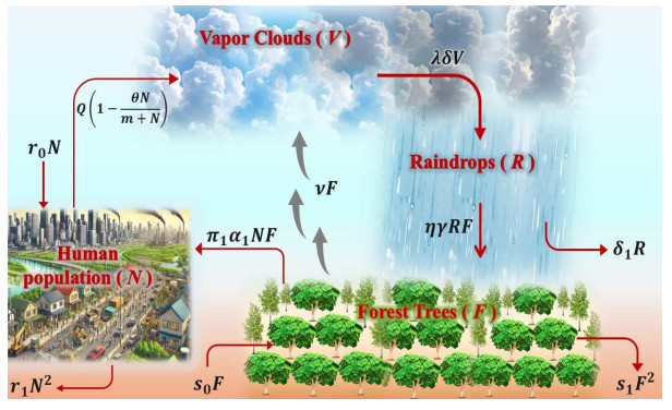
The hydrologic cycle is increasingly disrupted due to the rising human population and the associated decline in forest trees. The rationale of this work was to address the disruption in the hydrologic cycle, which is caused by the dual adverse effects of human population growth: reducing forestry trees and diminishing clouds' formation. The proposed model assumes that the density of forestry trees decreases due to harvesting activities to fulfill the resource demands of human population. Additionally, it posits that the transpiration from forestry trees contributes to an increased density of vapor clouds' formation, while population growth adversely impacts the natural formation rate of vapor clouds. The model was analyzed by employing qualitative analysis, demonstrating the feasibility and stability of equilibrium solutions. Furthermore, to capture the consequences of environmental fluctuations on the model's dynamics, the proposed deterministic model was extended to a stochastic framework. The analytical and numerical work sought to provide the directives for understanding and mitigating the adverse effects of human activities on the hydrologic cycle, promoting sustainable practices to restore ecological equilibrium. Results of the model analysis reveal that an increase in human population leads to a decline in both rainfall and forestry trees. However, reforestation with high–transpiration tree species can mitigate rainfall decline and restore balance to the hydrologic cycle. Moreover, the maximum density of forest trees is achieved when the utility of rain by the forest trees and the natural formation of vapor clouds are maximal. Also, the minimal anthropogenic hindrance in reducing the natural formation of vapor clouds, combined with the maximal efficiency of vapor clouds to naturally convert into raindrops, facilitates maximum rainfall.

| [1] |
Z. Cui, Y. Zhang, A. Wang, J. Wu, Forest evapotranspiration trends and their driving factors under climate change, J. Hydrol., 644 (2024), 132114. https://doi.org/10.1016/j.jhydrol.2024.132114 doi: 10.1016/j.jhydrol.2024.132114

|
| [2] |
D. Sheil, How plants water our planet: Advances and imperatives, Trends Plant Sci., 19 (2014), 209–211. https://doi.org/10.1016/j.tplants.2014.01.002 doi: 10.1016/j.tplants.2014.01.002
|
| [3] |
S. Jasechko, Z. Sharp, J. Gibson, S. J. Birks, Y. Yi, P. J. Fawcett, Terrestrial water fluxes dominated by transpiration, Nature, 496 (2013), 347–350. https://doi.org/10.1038/nature11983 doi: 10.1038/nature11983
|
| [4] |
J. E. Bagley, A. R. Desai, K. J. Harding, P. K. Snyder, J. A. Foley, Drought and deforestation: Has land cover change influenced recent precipitation extremes in the Amazon?, J. Climate, 27 (2014), 345–361. https://doi.org/10.1175/JCLI-D-12-00369.1 doi: 10.1175/JCLI-D-12-00369.1
|
| [5] |
S. A. Spera, G. L. Galford, M. T. Coe, M. N. Macedo, J. F. Mustard, Land-use change affects water recycling in Brazil's last agricultural frontier, Glob. Chang. Biol., 22 (2016), 3405–3413. https://doi.org/10.1111/gcb.13298 doi: 10.1111/gcb.13298
|
| [6] |
A. Staal, O. A. Tuinenburg, J. H. C. Bosmans, M. Holmgren, E. H. V. Nes, M. Scheffer, et al., Forest–rainfall cascades buffer against drought across the Amazon, Nat. Clim. Change, 8 (2018), 539–543. https://doi.org/10.1038/s41558-018-0177-y doi: 10.1038/s41558-018-0177-y
|
| [7] |
R. Ranjan, Assessing the impact of mining on deforestation in India, Resour. Policy, 60 (2019), 23–35. https://doi.org/10.1016/j.resourpol.2018.11.022 doi: 10.1016/j.resourpol.2018.11.022
|
| [8] |
M. Bologna, G. Aquino, Deforestation and world population sustainability: A quantitative analysis, Sci. Rep., 10 (2020), 7631. https://doi.org/10.1038/s41598-020-63657-6 doi: 10.1038/s41598-020-63657-6
|
| [9] |
C. M. Jr Souza, J. V. Siqueira, M. H. Sales, A. V. Fonseca, J. G. Ribeiro, I. Numata, et al., Ten-year landsat classification of deforestation and forest degradation in the Brazilian Amazon, Remote Sens., 5 (2013), 5493–5513. https://doi.org/10.3390/rs5115493 doi: 10.3390/rs5115493
|
| [10] | FAO, Global Forest Resources Assessment 2020-Key findings. |
| [11] |
H. Boubekraoui, Y. Maouni, A. Ghallab, M. Draoui, A. Maouni, Spatio-temporal analysis and identification of deforestation hotspots in the Moroccan western Rif, Trees For. People, 12 (2023), 100388. https://dx.doi.org/10.2139/ssrn.4327300 doi: 10.2139/ssrn.4327300
|
| [12] |
C. Smith, J. C. Baker, D. V. Spracklen, Tropical deforestation causes large reductions in observed precipitation, Nature, 615 (2023), 270–275. https://doi.org/10.1038/s41586-022-05690-1 doi: 10.1038/s41586-022-05690-1
|
| [13] |
F. DeSales, T. Santiago, T. W. Biggs, K. Mullan, E. O. Sills, C. Monteverde, Impacts of protected area deforestation on dry-season regional climate in the Brazilian Amazon, J. Geophys. Res. Atmos., 125 (2020), e2020JD033048 https://doi.org/10.1029/2020JD033048 doi: 10.1029/2020JD033048
|
| [14] |
Y. Mu, T. W. Biggs, F. De Sales, Forests mitigate drought in an agricultural region of the Brazilian Amazon: Atmospheric moisture tracking to identify critical source areas, Geophys. Res. Lett., 48 (2021), e2020GL091380. https://doi.org/10.1029/2020GL091380 doi: 10.1029/2020GL091380
|
| [15] | H. Douville, K. Raghavan, J. Renwick, R. P. Allan, P. A. Arias, M. Barlow, et al., Water cycle changes, in Climate Change 2021: The Physical Science Basis, (2023), 1055–1210. |
| [16] | M. Kravcik, J. Lambert, A global action plan for the restoration of natural water cycles and climate, 2017. Avaiable from: https://bio4climate.org/downloads/Kravcik_Global_Action_Plan.pdf. |
| [17] |
B. Bhagowati, K. U. Ahamad, A review on lake eutrophication dynamics and recent developments in lake modeling, Ecohydrol. Hydrobiol., 19 (2019), 155–166. https://doi.org/10.1016/j.ecohyd.2018.03.002 doi: 10.1016/j.ecohyd.2018.03.002
|
| [18] |
D. Han, M. J. Currell, G. Cao, B. Hall, Alterations to groundwater recharge due to anthropogenic landscape change, J. Hydrol., 554 (2017), 545–557. https://doi.org/10.1016/j.jhydrol.2017.09.018 doi: 10.1016/j.jhydrol.2017.09.018
|
| [19] | E. Bilgic, A. Baba, Effect of urbanization on water resources: Challenges and prospects, in Groundwater in Arid and Semi-Arid Areas, Springer, (2023), 81–108. |
| [20] |
T. T. Vo, L. Hu, L. Xue, Q. Li, S. Chen, Urban effects on local cloud patterns, Proc. Natl. Acad. Sci., 120 (2023), e2216765120. https://doi.org/10.1073/pnas.2216765120 doi: 10.1073/pnas.2216765120
|
| [21] |
B. Dubey, S. Sharma, P. Sinha, J. B. Shukla, Modelling the depletion of forestry resources by population and population pressure augmented industrialization, Appl. Math. Modell., 33 (2009), 3002–3014. https://doi.org/10.1016/j.apm.2008.10.028 doi: 10.1016/j.apm.2008.10.028
|
| [22] |
K. Lata, A. K. Misra, J. B. Shukla, Modeling the effect of deforestation caused by human population pressure on wildlife species, Nonlinear Anal. Modell. Control, 23 (2018), 303–320. https://doi.org/10.15388/NA.2018.3.2 doi: 10.15388/NA.2018.3.2
|
| [23] |
K. Lata, A. K. Misra, The influence of forestry resources on rainfall: A deterministic and stochastic model, Appl. Math. Modell., 81 (2020), 673–689. https://doi.org/10.1016/j.apm.2020.01.009 doi: 10.1016/j.apm.2020.01.009
|
| [24] |
O. G. Gaoue, C. N. Ngonghala, J. Jiang, M. Lelu, Towards a mechanistic understanding of the synergistic effects of harvesting timber and non-timber forest products, Methods Ecol. Evol., 7 (2016), 398–406. https://doi.org/10.1111/2041-210X.12493 doi: 10.1111/2041-210X.12493
|
| [25] |
E. Karesdotter, G. Destouni, N. Ghajarnia, R.B. Lammers, Z. Kalantari, Distinguishing direct human-driven effects on the global terrestrial water cycle, Earth's Future, 10 (2022), e2022EF002848. https://doi.org/10.1029/2022EF002848 doi: 10.1029/2022EF002848
|
| [26] |
L. Tanika, C. Wamucii, L. Best, E. G. Lagneaux, M. Githinji, M. V. Noordwijk, Who or what makes rainfall? Relational and instrumental paradigms for human impacts on atmospheric water cycling, Curr. Opin. Environ. Sustain., 63 (2023), 101300. https://doi.org/10.1016/j.cosust.2023.101300 doi: 10.1016/j.cosust.2023.101300
|
| [27] |
A. K. Misra, G. Agrawal, K. Lata, Modeling the influence of human population and human population augmented pollution on rainfall, Discrete Continuous Dyn. Syst. Ser. B, 27 (2022), 2979–3003. https://doi.org/10.3934/dcdsb.2021169 doi: 10.3934/dcdsb.2021169
|
| [28] |
G. Agrawal, A. K. Agrawal, A. K. Misra, Modeling the impacts of chemical substances and time delay to mitigate regional atmospheric pollutants and enhance rainfall, Phys. D Nonlinear Phenom., 472 (2025), 134507. https://doi.org/10.1016/j.physd.2024.134507 doi: 10.1016/j.physd.2024.134507
|
| [29] |
S. Sundar, R. Naresh, A. K. Misra, J. B. Shukla, A nonlinear mathematical model to study the interactions of hot gases with cloud droplets and raindrops, Appl. Math. Modell., 33 (2009), 3015–3024. https://doi.org/10.1016/j.apm.2008.10.032 doi: 10.1016/j.apm.2008.10.032
|
| [30] |
Z. Huang, Q. Yang, J. Cao, A stochastic model for interactions of hot gases with cloud droplets and raindrops, Nonlinear Anal. Real World Appl., 12 (2011), 203–214. https://doi.org/10.1016/j.nonrwa.2010.06.008 doi: 10.1016/j.nonrwa.2010.06.008
|
| [31] | G. Agrawal, A. K. Agrawal, J. Dhar, Effects of human population and atmospheric pollution on rainfall: A modeling study, J. Indian Math. Soc., 91 (2024), 550–664. |
| [32] |
A. K. Misra, A. Tripathi, Stochastic stability of aerosols–stimulated rainfall model, Phys. A, 527 (2019), 121337. https://doi.org/10.1016/j.physa.2019.121337 doi: 10.1016/j.physa.2019.121337
|
| [33] |
G. Agrawal, A. K. Agrawal, J. Dhar, A. K. Misra, Modeling the impact of cloud seeding to rescind the effect of atmospheric pollutants on natural rainfall, Model. Earth Syst. Environ., 10 (2024), 1573–1588. https://doi.org/10.1007/s40808-023-01854-8 doi: 10.1007/s40808-023-01854-8
|
| [34] | A. K. Misra, G. Agrawal, A. Yadav, When to perform cloud seeding for maximum agricultural crop yields? A modeling study, Int. J. Numer. Methods Heat Fluid Flow, Forthcoming 2024. https://doi.org/10.1108/HFF-09-2024-0711 |
| [35] |
C. Salas-Eljatib, L. Mehtatalo, T. G. Gregoire, D. P. Soto, R. Vargas-Gatete, Growth equations in forest research: Mathematical basis and model similarities, Curr. Forestry Rep., 7 (2021), 230–244. https://doi.org/10.1007/s40725-021-00145-8 doi: 10.1007/s40725-021-00145-8
|
| [36] | F. Brauer, C. Castillo-Chavez, Mathematical Models in Population Biology and Epidemiology, Springer New York, 2011. https://doi.org/10.1007/978-1-4614-1686-9 |
| [37] | R. A. Houze, Chapter 3-Cloud microphysics, Int. Geophys., 104 (2014), 47–76. https://doi.org/10.1016/B978-0-12-374266-7.00003-2. |
| [38] | O. Boucher, Atmospheric Aerosols: Properties and Climate Impacts, Springer Dordrecht, Springer Nature, 2015. https://doi.org/10.1007/978-94-017-9649-1. |
| [39] |
M. O. Andreae, D. Rosenfeld, Aerosol-cloud-precipitation interactions. Part 1. The nature and sources of cloud-active aerosols, Earth-Sci. Rev., 89 (2008), 13–41. https://doi.org/10.1016/j.earscirev.2008.03.001 doi: 10.1016/j.earscirev.2008.03.001
|
| [40] |
M. Ruiz-Vasquez, P. A. Arias, J. A. Martinez, J. C. Espinoza, Effects of Amazon basin deforestation on regional atmospheric circulation and water vapor transport towards tropical South America, Clim. Dyn., 54 (2020), 4169–4189. https://doi.org/10.1007/s00382-020-05223-4 doi: 10.1007/s00382-020-05223-4
|
| [41] |
A. T. Leite-Filho, B. S. Soares-Filho, J. L. Davis, G. M. Abrahao, J. Borner, Deforestration reduces rainfall and agricultural revenues in the Brazilian Amazon, Nat. Commun., 12 (2021), 2591. https://doi.org/10.1038/s41467-021-22840-7 doi: 10.1038/s41467-021-22840-7
|
| [42] |
A. M. Makarieva, A. V. Nefiodov, A. D. Nobre, D. Sheil, P. Nobre, J. Pokorny, et al., Vegetation impact on atmospheric moisture transport under increasing land-ocean temperature contrasts, Heliyon, 8 (2022), e11173. https://doi.org/10.1016/j.heliyon.2022.e11173 doi: 10.1016/j.heliyon.2022.e11173
|
| [43] |
H. I. Freedman, J. W. H. So, Global stability and persistence of simple food chains, Math. Biosci., 76 (1985), 69–86. https://doi.org/10.1016/0025-5564(85)90047-1 doi: 10.1016/0025-5564(85)90047-1
|
| [44] | J. K. Hale, Ordinary Differential Equations, Wiley-Interscience, New York, 1969. |
| [45] |
Z. Huang, G. Huang, Mathematical analysis on deterministic and stochastic lake ecosystem models, Math. Biosci. Eng., 16 (2019), 4723–4740. https://doi.org/10.3934/mbe.2019237 doi: 10.3934/mbe.2019237
|
| [46] |
D. Bolatova, S. Kadyrov, A. Kashkynbayev, Mathematical modeling of infectious diseases and the impact of vaccination strategies, Math. Biosci. Eng., 21 (2024), 7103–7123. https://doi.org/10.3934/mbe.2024314 doi: 10.3934/mbe.2024314
|
| [47] |
S. Li, S. Wang, Analysis of a stochastic predator–prey model with disease in the predator and Beddington–DeAngelis functional response, Adv. Differ. Equations, 224 (2015). https://doi.org/10.1186/s13662-015-0448-0 doi: 10.1186/s13662-015-0448-0
|
| [48] | X. Mao, Stochastic Differential Equations and Applications, Horwood, New York, 1997. |
| [49] |
R. K. Upadhyay, R. D. Parshad, K. Antwi-Fordjour, E. Quansah, S. Kumari, Global dynamics of stochastic predator-prey model with mutual interference and prey defense, J. Appl. Math. Comput., 60 (2019), 169–190. https://doi.org/10.1007/s12190-018-1207-7 doi: 10.1007/s12190-018-1207-7
|
| [50] |
D. J. Higham, An algorithmic introduction to numerical simulation of stochastic differential equations, SIAM Rev., 43 (2001), 525–546. https://doi.org/10.1137/S0036144500378302 doi: 10.1137/S0036144500378302
|
| [51] |
X. Mao, G. Marion, E. Renshaw, Environmental Brownian noise suppresses explosions in population dynamics, Stochastic Process. Appl., 97 (2002), 95–110. https://doi.org/10.1016/S0304-4149(01)00126-0 doi: 10.1016/S0304-4149(01)00126-0
|
| [52] |
N. Dalal, D. Greenhalgh, X. Mao, A stochastic model for internal HIV dynamics, J. Math. Anal. Appl., 341 (2008), 1084–1101. https://doi.org/10.1016/j.jmaa.2007.11.005 doi: 10.1016/j.jmaa.2007.11.005
|
| [53] | L. Arnold, Stochastic Differential Equations: Theory and Applications, New York, 1974. |
| [54] | A. Friedman, Stochastic Differential Equations and Applications, Academic Press, New York, 1976. |


Figures(11) / Tables(1)

Gauri Agrawal, Alok Kumar Agrawal, Arvind Kumar Misra. Effects of human population and forestry trees on the hydrologic cycle: A modeling-based study[J]. Mathematical Biosciences and Engineering, 2025, 22(8): 2072-2104. doi: 10.3934/mbe.2025076


 DownLoad: