Predicting the transmission trends of COVID-19: an interpretable machine learning approach based on daily, death, and imported cases

Hyeonjeong Ahn; Hyojung Lee; Hyeonjeong Ahn; Hyojung Lee

doi:10.3934/mbe.2024270

Mathematical Biosciences and Engineering

2024, Volume 21, Issue 5: 6150-6166. doi: 10.3934/mbe.2024270

Previous Article Next Article

Research article

Predicting the transmission trends of COVID-19: an interpretable machine learning approach based on daily, death, and imported cases

Hyeonjeong Ahn ,
Hyojung Lee ^,

Department of Statistics, Kyungpook National University, Daegu 41566, Republic of Korea

Academic Editor: Xi Huo

Received: 14 January 2024 Revised: 21 May 2024 Accepted: 29 May 2024 Published: 03 June 2024

COVID-19 is caused by the SARS-CoV-2 virus, which has produced variants and increasing concerns about a potential resurgence since the pandemic outbreak in 2019. Predicting infectious disease outbreaks is crucial for effective prevention and control. This study aims to predict the transmission patterns of COVID-19 using machine learning, such as support vector machine, random forest, and XGBoost, using confirmed cases, death cases, and imported cases, respectively. The study categorizes the transmission trends into the three groups: L0 (decrease), L1 (maintain), and L2 (increase). We develop the risk index function to quantify changes in the transmission trends, which is applied to the classification of machine learning. A high accuracy is achieved when estimating the transmission trends for the confirmed cases (91.5–95.5%), death cases (85.6–91.8%), and imported cases (77.7–89.4%). Notably, the confirmed cases exhibit a higher level of accuracy compared to the data on the deaths and imported cases. L2 predictions outperformed L0 and L1 in all cases. Predicting L2 is important because it can lead to new outbreaks. Thus, this robust L2 prediction is crucial for the timely implementation of control policies for the management of transmission dynamics.
- COVID-19,
- machine learning,
- transmission,
- classification,
- prediction
Citation: Hyeonjeong Ahn, Hyojung Lee. Predicting the transmission trends of COVID-19: an interpretable machine learning approach based on daily, death, and imported cases[J]. Mathematical Biosciences and Engineering, 2024, 21(5): 6150-6166. doi: 10.3934/mbe.2024270

Related Papers:

Abstract

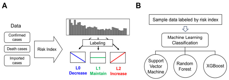
COVID-19 is caused by the SARS-CoV-2 virus, which has produced variants and increasing concerns about a potential resurgence since the pandemic outbreak in 2019. Predicting infectious disease outbreaks is crucial for effective prevention and control. This study aims to predict the transmission patterns of COVID-19 using machine learning, such as support vector machine, random forest, and XGBoost, using confirmed cases, death cases, and imported cases, respectively. The study categorizes the transmission trends into the three groups: L0 (decrease), L1 (maintain), and L2 (increase). We develop the risk index function to quantify changes in the transmission trends, which is applied to the classification of machine learning. A high accuracy is achieved when estimating the transmission trends for the confirmed cases (91.5–95.5%), death cases (85.6–91.8%), and imported cases (77.7–89.4%). Notably, the confirmed cases exhibit a higher level of accuracy compared to the data on the deaths and imported cases. L2 predictions outperformed L0 and L1 in all cases. Predicting L2 is important because it can lead to new outbreaks. Thus, this robust L2 prediction is crucial for the timely implementation of control policies for the management of transmission dynamics.

References

[1]	E. D. Wit, N. V. Doremalen, D. Falzarano, V. J. Munster, SARS and MERS: recent insights into emerging coronaviruses, Nat. Rev. Microbiol., 14 (2016), 523–534. https://doi.org/10.1038/nrmicro.2016.81 doi: 10.1038/nrmicro.2016.81
[2]	H. Nishiura, C. Castillo-Chavez, M. Safan, G. Chowell, Transmission potential of the new influenza A (H1N1) virus and its age-specificity in Japan, Eurosurveillance, 14 (2009), 19227. https://doi.org/10.2807/ese.14.22.19227-en doi: 10.2807/ese.14.22.19227-en
[3]	D. V. Parums, Editorial: A rapid global increase in COVID-19 is due to the emergence of the EG.5 (Eris) subvariant of omicron SARS-CoV-2, Med. Sci. Monit., 29 (2023), e942244. https://doi.org/10.12659/MSM.942244 doi: 10.12659/MSM.942244
[4]	C. Chakraborty, M. Bhattacharya, H. Chopra, M. A. Islam, G. Saikumar, K. Dhama, The SARS-CoV-2 Omicron recombinant subvariants XBB, XBB.1, and XBB.1.5 are expanding rapidly with unique mutations, antibody evasion, and immune escape properties—an alarming global threat of a surge in COVID-19 cases again?, Int. J. Surg., 109 (2023), 1041–1043. https://doi.org/10.1097/JS9.0000000000000246 doi: 10.1097/JS9.0000000000000246
[5]	M. Coccia, Sources, diffusion and prediction in COVID-19 pandemic: lessons learned to face next health emergency, AIMS Public Health, 10 (2023), 145–168. https://doi.org/10.3934/publichealth.2023012 doi: 10.3934/publichealth.2023012
[6]	G. Cho, J. R. Park, Y. Choi, H. Ahn, H. Lee, Detection of COVID-19 epidemic outbreak using machine learning, Front. Public Health, 11 (2023), 1252357. https://doi.org/10.3389/fpubh.2023.1252357 doi: 10.3389/fpubh.2023.1252357
[7]	A. Dairi, F. Harrou, A. Zeroual, M. M. Hittawe, Y. Sun, Comparative study of machine learning methods for COVID-19 transmission forecasting, J. Biomed. Inf., 118 (2021), 103791. https://doi.org/10.1016/j.jbi.2021.103791 doi: 10.1016/j.jbi.2021.103791
[8]	H. Kang, K. D. Min, S. Jeon, J. Y. Lee, S. I. Cho, A measure to estimate the risk of imported COVID-19 cases and its application for evaluating travel-related control measures, Sci. Rep., 12 (2022), 9497. https://doi.org/10.1038/s41598-022-13775-0 doi: 10.1038/s41598-022-13775-0
[9]	W. C. Wang, T. Y. Lin, S. Y. Chiu, C. N. Chen, P. Sarakarn, M. Ibrahim, et al., Classification of community-acquired outbreaks for the global transmission of COVID-19: Machine learning and statistical model analysis, J. Formosan Med. Assoc., 120 (2021), S26–S37. https://doi.org/10.1016/j.jfma.2021.05.010 doi: 10.1016/j.jfma.2021.05.010
[10]	S. G. Paul, A. Saha, A. A. Biswas, M. S. Zulfiker, M. S. Arefin, M. M. Rahman, et al., Combating COVID-19 using machine learning and deep learning: Applications, challenges, and future perspectives, Array, 17 (2023), 100271. https://doi.org/10.1016/j.array.2022.100271 doi: 10.1016/j.array.2022.100271
[11]	G. Cho, Y. J. Kim, S. H. Seo, G. Jang, H. Lee, Cost-effectiveness analysis of COVID-19 variants effects in an age-structured model, Sci. Rep., 13 (2023), 15844. https://doi.org/10.1038/s41598-023-41876-x doi: 10.1038/s41598-023-41876-x
[12]	W. D. de Holanda, L. C. e Silva, Á . A. C. C. Sobrinho, Machine learning models for predicting hospitalization and mortality risks of COVID-19 patients, Expert Syst. Appl., 240 (2024), 122670. https://doi.org/10.1016/j.eswa.2023.122670 doi: 10.1016/j.eswa.2023.122670
[13]	S. Kim, Y. Ko, Y. J. Kim, E. Jung, The impact of social distancing and public behavior changes on COVID-19 transmission dynamics in the Republic of Korea, PLoS One, 15 (2020), e0238684. https://doi.org/10.1371/journal.pone.0238684 doi: 10.1371/journal.pone.0238684
[14]	A. Olivares, E. Staffetti, Optimal control-based vaccination and testing strategies for COVID-19, Comput. Methods Programs Biomed., 211 (2021), 106411. https://doi.org/10.1016/j.cmpb.2021.106411 doi: 10.1016/j.cmpb.2021.106411
[15]	S. Agrebi, A. Larbi, Use of artificial intelligence in infectious diseases, in Artificial Intelligence in Precision Health, (2020), 415–438. https://doi.org/10.1016/B978-0-12-817133-2.00018-5
[16]	F. Wong, C. de la Fuente-Nunez, J. J. Collins, Leveraging artificial intelligence in the fight against infectious diseases, Science, 381 (2023), 164–170. https://doi.org/10.1126/science.adh1114 doi: 10.1126/science.adh1114
[17]	V. K. R. Chimmula, L. Zhang, Time series forecasting of COVID-19 transmission in Canada using LSTM networks, Chaos Solitons Fractals, 135 (2020), 109864. https://doi.org/10.1016/j.chaos.2020.109864 doi: 10.1016/j.chaos.2020.109864
[18]	I. Sardar, M. A. Akbar, V. Leiva, A. Alsanad, P. Mishra, Machine learning and automatic ARIMA/Prophet models-based forecasting of COVID-19: methodology, evaluation, and case study in SAARC countries, Stochastic Environ. Res. Risk Assess., 37 (2023), 345–359. https://doi.org/10.1007/s00477-022-02307-x doi: 10.1007/s00477-022-02307-x
[19]	E. Gothai, R. Thamilselvan, R. R. Rajalaxmi, R. M. Sadana, A. Ragavi, R. Sakthivel, Prediction of COVID-19 growth and trend using machine learning approach, Mater. Today Proc., 81 (2023), 597–601. https://doi.org/10.1016/j.matpr.2021.04.051 doi: 10.1016/j.matpr.2021.04.051
[20]	I. Heredia Cacha, J. Sainz-Pardo Diaz, M. Castrillo, A. Lopez Garcia, Forecasting COVID-19 spreading through an ensemble of classical and machine learning models: Spain's case study, Sci. Rep., 13 (2023), 6750. https://doi.org/10.1038/s41598-023-33795-8 doi: 10.1038/s41598-023-33795-8
[21]	P. Ramazi, A. Haratian, M. Meghdadi, A. Mari Oriyad, M. A. Lewis, Z. Maleki, et al., Accurate long-range forecasting of COVID-19 mortality in the USA, Sci. Rep., 11 (2021), 13822. https://doi.org/10.1038/s41598-021-91365-2 doi: 10.1038/s41598-021-91365-2
[22]	K. Moulaei, M. Shanbehzadeh, Z. Mohammadi-Taghiabad, H. Kazemi-Arpanahi, Comparing machine learning algorithms for predicting COVID-19 mortality, BMC Med. Inf. Decis. Making, 22 (2022), 2. https://doi.org/10.1186/s12911-021-01742-0 doi: 10.1186/s12911-021-01742-0
[23]	F. Rustam, A. A. Reshi, A. Mehmood, S. Ullah, B. W. On, W. Aslam, et al., COVID-19 future forecasting using supervised machine learning models, IEEE Access, 8 (2020), 101489–101499. https://doi.org/10.1109/access.2020.2997311 doi: 10.1109/access.2020.2997311
[24]	E. Y. Alqaissi, F. S. Alotaibi, M. S. Ramzan, Modern machine-learning predictive models for diagnosing infectious diseases, Comput. Math. Methods Med., 2022 (2022), 6902321. https://doi.org/10.1155/2022/6902321 doi: 10.1155/2022/6902321
[25]	N. M. Tayarani, Applications of artificial intelligence in battling against COVID-19: A literature review, Chaos Solitons Fractals, 142 (2021), 110338. https://doi.org/10.1016/j.chaos.2020.110338 doi: 10.1016/j.chaos.2020.110338
[26]	Korea Disease Control and Prevention (KDCA), Open Source Data for COVID-19, 2023. Available from: https://dportal.kdca.go.kr/pot/cv/trend/dmstc/selectMntrgSttus.do.
[27]	CoVariant, Overview of Variants in Countries, 2023. Available from: https://covariants.org/per-country.
[28]	H. Zhao, N. N. Merchant, A. McNulty, T. A. Radcliff, M. J. Cote, R. S. B. Fischer, et al., COVID-19: Short term prediction model using daily incidence data, PLoS One, 16 (2021), e0250110. https://doi.org/10.1371/journal.pone.0250110 doi: 10.1371/journal.pone.0250110
[29]	H. Du, E. Dong, H. S. Badr, M. E. Petrone, N. D. Grubaugh, L. M. Gardner, Incorporating variant frequencies data into short-term forecasting for COVID-19 cases and deaths in the USA: a deep learning approach, EBioMedicine, 89 (2023), 104482. https://doi.org/10.1016/j.ebiom.2023.104482 doi: 10.1016/j.ebiom.2023.104482
[30]	T. Usherwood, Z. LaJoie, V. Srivastava, A model and predictions for COVID-19 considering population behavior and vaccination, Sci. Rep., 11 (2021), 12051. https://doi.org/10.1038/s41598-021-91514-7 doi: 10.1038/s41598-021-91514-7
[31]	H. Lee, Y. Kim, E. Kim, S. Lee, Risk assessment of importation and local transmission of COVID-19 in South Korea: Statistical modeling approach, JMIR Public Health Surveillance, 7 (2021), e26784. https://doi.org/10.2196/26784 doi: 10.2196/26784
[32]	S. B. Keser, K. Keskin, A gradient boosting-based mortality prediction model for COVID-19 patients, Neural Comput. Appl., 35 (2023), 23997–24013. https://doi.org/10.1007/s00521-023-08997-w doi: 10.1007/s00521-023-08997-w
[33]	D. Chumachenko, I. Meniailov, K. Bazilevych, T. Chumachenko, S. Yakovlev, Investigation of statistical machine learning models for COVID-19 epidemic process simulation: Random forest, K-nearest neighbors, gradient boosting, Computation, 10 (2022), 86. https://doi.org/10.3390/computation10060086 doi: 10.3390/computation10060086
[34]	S. Ardabili, A. Mosavi, P. Ghamisi, F. Ferdinand, A. Varkonyi-Koczy, U. Reuter, et al., COVID-19 outbreak prediction with machine learning, Algorithms, 13 (2020), 249. https://doi.org/10.3390/a13100249 doi: 10.3390/a13100249
[35]	F. Shahid, A. Zameer, M. Muneeb, Predictions for COVID-19 with deep learning models of LSTM, GRU and Bi-LSTM, Chaos Solitons Fractals, 140 (2020), 110212. https://doi.org/10.1016/j.chaos.2020.110212 doi: 10.1016/j.chaos.2020.110212
[36]	A. K. Srivastava, S. M. Tripathi, S. Kumar, R. M. Elavarasan, S. Gangatharan, D. Kumar, et al., Machine learning approach for forecast analysis of novel COVID-19 scenarios in India, IEEE Access, 10 (2022), 95106–95124. https://doi.org/10.1109/access.2022.3204804 doi: 10.1109/access.2022.3204804
[37]	Y. Alali, F. Harrou, Y. Sun, A proficient approach to forecast COVID-19 spread via optimized dynamic machine learning models, Sci. Rep., 12 (2022), 2467. https://doi.org/10.1038/s41598-022-06218-3 doi: 10.1038/s41598-022-06218-3

mbe-21-05-270-ESM.pdf

Reader Comments

Your name:*

Email:*
© 2024 the Author(s), licensee AIMS Press. This is an open access article distributed under the terms of the Creative Commons Attribution License (http://creativecommons.org/licenses/by/4.0)