A kinetic model considering the decline of antibody level and simulation about vaccination effect of COVID-19

Chuanqing Xu; Xiaotong Huang; Zonghao Zhang; Jing'an Cui; Chuanqing Xu; Xiaotong Huang; Zonghao Zhang; Jing'an Cui

doi:10.3934/mbe.2022586

Mathematical Biosciences and Engineering

2022, Volume 19, Issue 12: 12558-12580. doi: 10.3934/mbe.2022586

Previous Article Next Article

Research article Special Issues

A kinetic model considering the decline of antibody level and simulation about vaccination effect of COVID-19

School of Science, Beijing University of Civil Engineering and Architecture, China

Received: 14 December 2021 Revised: 24 April 2022 Accepted: 26 July 2022 Published: 29 August 2022

We build a model that consider the falling antibody levels and vaccination to assess the impact of falling antibody levels and vaccination on the spread of the COVID-19 outbreak, and simulate the influence of vaccination rates and failure rates on the number of daily new cases in England. We get that the lower the vaccine failure rate, the fewer new cases. Over time, vaccines with low failure rates are more effective in reducing the number of cases than vaccines with high failure rates and the higher the vaccine efficiency and vaccination rate, the lower the epidemic peak. The peak arrival time is related to a boundary value. When the failure rate is less than this boundary value, the peak time will advance with the decrease of failure rate; when the failure rate is greater than this boundary value, the peak time is delayed with the decrease of failure rate. On the basis of improving the effectiveness of vaccines, increasing the vaccination rate has practical significance for controlling the spread of the epidemic.
- COVID-19,
- epidemic dynamics,
- SEIR model,
- vaccine efficiency
Citation: Chuanqing Xu, Xiaotong Huang, Zonghao Zhang, Jing'an Cui. A kinetic model considering the decline of antibody level and simulation about vaccination effect of COVID-19[J]. Mathematical Biosciences and Engineering, 2022, 19(12): 12558-12580. doi: 10.3934/mbe.2022586

Related Papers:

Abstract

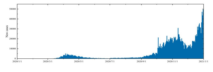
We build a model that consider the falling antibody levels and vaccination to assess the impact of falling antibody levels and vaccination on the spread of the COVID-19 outbreak, and simulate the influence of vaccination rates and failure rates on the number of daily new cases in England. We get that the lower the vaccine failure rate, the fewer new cases. Over time, vaccines with low failure rates are more effective in reducing the number of cases than vaccines with high failure rates and the higher the vaccine efficiency and vaccination rate, the lower the epidemic peak. The peak arrival time is related to a boundary value. When the failure rate is less than this boundary value, the peak time will advance with the decrease of failure rate; when the failure rate is greater than this boundary value, the peak time is delayed with the decrease of failure rate. On the basis of improving the effectiveness of vaccines, increasing the vaccination rate has practical significance for controlling the spread of the epidemic.

References

[1]	D. Wang, B. Hu, C. Hu, F. Zhu, X. Liu, J. Zhang, et al., Clinical characteristics of 138 hospitalized patients with 2019 novel coronavirus–infected pneumonia in Wuhan, China, JAMA, 323 (2020), 1061–1069. https://doi.org/10.1001/jama.2020.1585 doi: 10.1001/jama.2020.1585
[2]	N. Zhu, D. Zhang, W. Wang, X. Li, B. Yang, J. Song, et al., A novel coronavirus from patients with pneumonia in China, 2019, N. Engl. J. Med, 382 (2020), 727–733. https://doi.org/10.1056/NEJMoa200101 doi: 10.1056/NEJMoa200101
[3]	T. Guo, Q. Shen, W. Guo, W. He, J. Li, Y. Zhang, et al., Clinical characteristics of elderly patients with Covid-19 in Hunan province, China: a multicenter, retrospective study, Gerontology, 66 (2020), 1–9. https://doi.org/10.1159/000508734 doi: 10.1159/000508734
[4]	UCLA, Scientists Discover How COVID-19 Virus Causes Multiple Organ Failure in Mice, 2020. Available from: https://newsroom.ucla.edu/releases/covid-19-multiple-organ-failure-systemic-effects.
[5]	World Health Organization, WHO Coronavirus (COVID-19) Dashboard, 2021. Available from: https://covid19.who.int/.
[6]	GOV.UK, Coronavirus (COVID-19) in the UK, 2020. Available from: https://coronavirus.data.gov.uk/details/cases.
[7]	Imperial College London, Coronavirus Antibody Prevalence Falling in England, REACT Study Shows, 2021. Available from: https://www.imperial.ac.uk/news/207333/coronavirus-antibody-prevalence-falling-england-react/.
[8]	Q. Long, X. Tang, Q. Shi, Q. Li, H. Deng, J. Yuan, et al., Clinical and immunological assessment of asymptomatic SARS-CoV-2 infections, Nat. Med., 26 (2020), 1200–1204. https://doi.org/10.1038/s41591-020-0965-6 doi: 10.1038/s41591-020-0965-6
[9]	J. Seow, C. Graham, B. Merrick, S. Acors, S. Pickering, K. J. A. Steel, et al., Longitudinal observation and decline of neutralizing antibody responses in the three months following SARS-CoV-2 infection in humans, Nat. Microbiol., 5 (2020), 1598–1607. https://doi.org/10.1038/s41564-020-00813-8 doi: 10.1038/s41564-020-00813-8
[10]	P. Mlcochova, S. Kemp, M. S. Dhar, G. Papa, B. Meng, S. Mishra, et al., SARS-CoV-2 B.1.617.2 Delta variant replication and immune evasion, Nature, 599 (2021), 114–119. https://doi.org/10.1038/s41586-021-03944-y doi: 10.1038/s41586-021-03944-y
[11]	P. D. Yadav, G. N. Sapkal, E. Raches, R. R. Sahay, D. A. Nyayanit, D. Y. Patil, et al., Neutralization of Beta and Delta variant with sera of COVID-19 recovered cases and vaccines of inactivated COVID-19 vaccine BBV152/Covaxin, J. Travel. Med., 28 (2021), 1195–1982. https://doi.org/10.1093/jtm/taab104 doi: 10.1093/jtm/taab104
[12]	D. Planas, D. Veyer, A. Baidaliuk, I. Staropoli, F. Guivel-Benhassine, M. M. Rajahet, et al., Reduced sensitivity of SARS-CoV-2 variant Delta to antibody neutralization, Nature, 596 (2021), 276–280. https://doi.org/10.1038/s41586-021-03777-9 doi: 10.1038/s41586-021-03777-9
[13]	P. Wintachai, K. Prathom, Stability analysis of SEIR model related to efficiency of vaccines for COVID-19 situation, Heliyon, 7 (2021), e06812. https://doi.org/10.1016/j.heliyon.2021.e06812 doi: 10.1016/j.heliyon.2021.e06812
[14]	A. Fuady, N. Nuraini, K. K. Sukandar, B. W. Lestari, Targeted vaccine allocation could increase the COVID-19 vaccine benefifits amidst its lack of availability: A mathematical modeling study in Indonesia, Vaccines, 9 (2021), 050462. https://doi.org/10.3390/VACCINES9050462 doi: 10.3390/VACCINES9050462
[15]	M. Angeli, G. Neofotistos, M. Mattheakis, E. Kaxiras, Modeling the effect of the vaccination campaign on the COVID-19 pandemic, Chaos, Solitons Fractals, 154 (2022), 111621. https://doi.org/10.1016/j.chaos.2021.111621 doi: 10.1016/j.chaos.2021.111621
[16]	S. Zhai, G. Luo, T. Huang, X. Wang, J. Tao, P. Zhou, Vaccination control of an epidemic model with time delay and its application to COVID-19, Nonlinear Dyn., 106 (2021), 1279–1292. https://doi.org/10.1007/s11071-021-06533-w doi: 10.1007/s11071-021-06533-w
[17]	J. Medina, R. Cessa-Rojas, V. Umpaichitra, Reducing COVID-19 cases and deaths by applying blockchain in vaccination rollout management, IEEE Open J. Engineer. Med. Biol., 2 (2021), 249–255. https://doi.org/10.1109/OJEMB.2021.3093774 doi: 10.1109/OJEMB.2021.3093774
[18]	A. Karabay, A. Kuzdeuov, S. Ospanova, M. Lewis, H. A. Varol, A vaccination simulator for COVID-19: Effective and sterilizing immunization cases, IEEE J. Biomed. Health Inf., 25 (2021), 4317–4327. https://doi.org/10.1109/JBHI.2021.3114180 doi: 10.1109/JBHI.2021.3114180
[19]	25th International Conference on System Theory, Control and Computing (ICSTCC), Simulation of SARS-CoV-2 Pandemic in Germany with Ordinary Differential Equations in MATLAB, 2021. Available from: https://doi.org/10.1109/ICSTCC52150.2021.9607181.
[20]	H. Chen, B. Haus, P. Mercorelli, Extension of SEIR compartmental models for constructive Lyapunov control of COVID-19 and analysis in terms of practical stability, Mathematics, 9 (2021), 172076. https://doi.org/10.3390/math9172076 doi: 10.3390/math9172076
[21]	P. V. D. Driessche, Reproduction numbers of infectious disease models, Infect. Dis. Model., 2 (2017), 288–303. https://doi.org/10.3390/math9172076 doi: 10.3390/math9172076
[22]	Y. Zhang, C. You, Z. Cai, J. Sun, W. Hu, X. Zhou, et al., Prediction of the COVID-19 outbreak based on a realistic stochastic model, preprint: https://doi.org/10.1101/2020.03.10.20033803.
[23]	Irish Examiner, Covid-19 Vaccination 'Incubation Period' for 10-14 Days before Second Dose, 2020. Available from: https://www.irishexaminer.com/world/arid-40198611.html.
[24]	The Emory Wheel, COVID-19 Cases Remain Steady after Two Weeks Mask Optional, 2022. Available from: https://emorywheel.com/covid-19-cases-remain-steady-after-two-weeks-mask-optional.
[25]	D. F. Gudbjartsson, G. L. Norddahl, P. Melsted, K. Gunnarsdottir, K. Stefansson, Humoral immune response to SARS-CoV-2 in iceland, New Engl. J. Med., 383 (2020), 1724–1734. https://doi.org/10.1056/NEJMoa2026116 doi: 10.1056/NEJMoa2026116
[26]	A. Longchamp, J. Longchamp, A. Croxatto, G. Greub, J. Delaloye, Serum antibody response in critically ill patients with COVID-19, Intensive Care Med., 46 (2020), 1921–1923. https://doi.org/10.1007/s00134-020-06171-7 doi: 10.1007/s00134-020-06171-7
[27]	GOV.CHN, News Analysis: As lockdown extends, Israel Faces Dilemma on How to Move Forward World Knowledge, 2021. Available from: http://www.china.org.cn/world/Off_the_Wire/2020-03/31/content_75878980.htm.
[28]	Worldometer, WORLD/COUNTRIES/ISRAEL, 2021. Available from: https://www.worldometers.info/coronavirus/country/israel/.

Reader Comments

Your name:*

Email:*
© 2022 the Author(s), licensee AIMS Press. This is an open access article distributed under the terms of the Creative Commons Attribution License (http://creativecommons.org/licenses/by/4.0)