The impact of intellectual property rights protection on green innovation: A quasi-natural experiment based on the pilot policy of the Chinese intellectual property court

Yue Liu; Liming Chen; Han Luo; Yuzhao Liu; Yixian Wen; Yue Liu; Liming Chen; Han Luo; Yuzhao Liu; Yixian Wen

doi:10.3934/mbe.2024114

Mathematical Biosciences and Engineering

2024, Volume 21, Issue 2: 2587-2607. doi: 10.3934/mbe.2024114

Previous Article Next Article

Research article Special Issues

The impact of intellectual property rights protection on green innovation: A quasi-natural experiment based on the pilot policy of the Chinese intellectual property court

Yue Liu ^{1
,
,},
Liming Chen ^{2
,
,},
Han Luo ³,
Yuzhao Liu ²,
Yixian Wen ¹

1.
Business School, Hunan Institute of Technology, Hengyang, Hunan Province, China
2.
School of Finance and Statistics, Hunan University, Changsha, Hunan Province, China
3.
Zhuzhou Branch of Hunan Tobacco Company, Zhuzhou, Hunan Province, China

Received: 22 December 2023 Revised: 10 January 2024 Accepted: 12 January 2024 Published: 18 January 2024

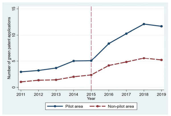
In the context of high-quality economic development in China, it is important to promote green innovation development by protecting intellectual property rights (IPR). Taking the pilot policy of the intellectual property courts in Beijing, Shanghai, and Guangzhou for example in a quasi-natural experiment, this article examines the effect of IPR protection on the development of corporate green innovation and its mechanisms by using a difference-in-differences model and a mediating effect model based on Chinese enterprise data from 2011 to 2019. The study found that first, IPR protection promotes enterprise green technological innovation; second, IPR protection affects green innovation through enterprise financing constraints and R&D investment; that is, increasing enterprise R&D investment and alleviating enterprise financing constraints are two important channels through which IPR protection promotes enterprise green technological innovation.
- intellectual property rights protection,
- green innovation,
- quasi-natural experiment,
- difference-in-differences model,
- ecological protection
Citation: Yue Liu, Liming Chen, Han Luo, Yuzhao Liu, Yixian Wen. The impact of intellectual property rights protection on green innovation: A quasi-natural experiment based on the pilot policy of the Chinese intellectual property court[J]. Mathematical Biosciences and Engineering, 2024, 21(2): 2587-2607. doi: 10.3934/mbe.2024114

Related Papers:

Abstract

In the context of high-quality economic development in China, it is important to promote green innovation development by protecting intellectual property rights (IPR). Taking the pilot policy of the intellectual property courts in Beijing, Shanghai, and Guangzhou for example in a quasi-natural experiment, this article examines the effect of IPR protection on the development of corporate green innovation and its mechanisms by using a difference-in-differences model and a mediating effect model based on Chinese enterprise data from 2011 to 2019. The study found that first, IPR protection promotes enterprise green technological innovation; second, IPR protection affects green innovation through enterprise financing constraints and R&D investment; that is, increasing enterprise R&D investment and alleviating enterprise financing constraints are two important channels through which IPR protection promotes enterprise green technological innovation.

References

[1]	Y. Hao, Z. Gai, G. Yan, H. Wu, M. Irfan, The spatial spillover effect and nonlinear relationship analysis between environmental decentralization, government corruption and air pollution: Evidence from China, Sci. Total Environ., 763 (2021), 144183. https://doi.org/10.1016/j.scitotenv.2020.144183
[2]	F. Allen, J. Qian, M. Qian, Law, finance, and economic growth in China, J. Financ. Econ., 77 (2004), 57–116. https://doi.org/10.1016/j.jfineco.2004.06.010 doi: 10.1016/j.jfineco.2004.06.010
[3]	X. B. Li, Behind the recent surge of Chinese patenting: An institutional view, Res. Policy, 41 (2011), 236–249. https://doi.org/10.1016/J.RESPOL.2011.07.003 doi: 10.1016/J.RESPOL.2011.07.003
[4]	L. Liu, M. Liu, How does the digital economy affect industrial eco-efficiency? Empirical evidence from China, Data Sci. Finance Econ., 2 (2022), 371–390. https://doi.org/10.3934/DSFE.2022019 doi: 10.3934/DSFE.2022019
[5]	Z. H. Li, J. H. Zhu, J. J. He, The effects of digital financial inclusion on innovation and entrepreneurship: A network perspective, Electron. Res. Arch., 30 (2022), 4697–4715. https://doi.org/10.3934/era.2022238 doi: 10.3934/era.2022238
[6]	A. Blackman, Z. Y. Li, A. A. Liu, Efficacy of command-and-control and market-based environmental regulation in developing countries, Annu. Rev. Resour. Econ., 10 (2018), 381–404. https://doi.org/10.1146/annurev-resource-100517-023144 doi: 10.1146/annurev-resource-100517-023144
[7]	M. Shugurov, International cooperation on climate research and green technologies in the face of sanctions: The case of Russia, Green Finance, 5 (2023), 102–153. https://doi.org/10.3934/GF.2023006 doi: 10.3934/GF.2023006
[8]	T. Lin, M. Y. Du, S. Y. Ren, How do green bonds affect green technology innovation? Firm evidence from China, Green Finance, 4 (2022), 492–511. https://doi.org/10.3934/GF.2022024 doi: 10.3934/GF.2022024
[9]	Y. Liu, P. Failler, Y. Ding, Enterprise financialization and technological innovation: Mechanism and heterogeneity, PLoS One, 17 (2022), e0275461. https://doi.org/10.1371/JOURNAL.PONE.0275461 doi: 10.1371/JOURNAL.PONE.0275461
[10]	X. Yang, J. Cao, Z. Liu, Y. Lai, Environmental policy uncertainty and green innovation: A TVP-VAR-SV model approach, Quant. Finance Econ., 6 (2022), 604–621. https://doi.org/10.3934/QFE.2022026 doi: 10.3934/QFE.2022026
[11]	Y. Liu, C. Ma, Z. H. Huang, Can the digital economy improve green total factor productivity? An empirical study based on Chinese urban data, Math. Biosci. Eng., 20 (2023), 6866–6893. https://doi.org/10.3934/mbe.2023296 doi: 10.3934/mbe.2023296
[12]	Z. Li, B. Mo, H. Nie, Time and frequency dynamic connectedness between cryptocurrencies and financial assets in China, Int. Rev. Econ. Finance, 86 (2023), 46–57. https://doi.org/10.1016/j.iref.2023.01.015 doi: 10.1016/j.iref.2023.01.015
[13]	P. Hsu, X. Tian, Y. Xu, Financial development and innovation: Cross-country evidence, J. Financ. Econ., 112 (2013), 116–135. https://doi.org/10.1016/j.jfineco.2013.12.002 doi: 10.1016/j.jfineco.2013.12.002
[14]	Y. M. Zhang, J. J. Zhang, Z. Cheng, Stock market liberalization and corporate green innovation: Evidence from China, Int. J. Environ. Res. Public Health, 18 (2021), 3412. https://doi.org/10.3390/ijerph18073412 doi: 10.3390/ijerph18073412
[15]	Z. Li, C. Yang, Z. Huang, How does the fintech sector react to signals from central bank digital currencies? Finance Res. Lett., 50 (2022), 103308.https://doi.org/10.1016/j.frl.2022.103308
[16]	Z. H. Li, G. K. Liao, Z. Z. Wang, Z. Huang, Green loan and subsidy for promoting clean production innovation, J Clean Prod., 187 (2018), 421–431. https://doi.org/10.1016/j.jclepro.2018.03.066 doi: 10.1016/j.jclepro.2018.03.066
[17]	Z. Li, Z. Huang, H. Dong, The influential factors on outward foreign direct investment: evidence from the "The Belt and Road", Emerging Mark. Finance Trade, 55 (2019), 3211–3226. https://doi.org/10.1080/1540496x.2019.1569512 doi: 10.1080/1540496x.2019.1569512
[18]	Y. Liu, Z. H. Li, M. R. Xu, The influential factors of financial cycle spillover: evidence from China, Emerging Mark. Finance Trade, 56 (2020), 1336–1350. https://doi.org/10.1080/1540496x.2019.1658076 doi: 10.1080/1540496x.2019.1658076
[19]	E. Dinopoulos, P. S. Segerstrom, Intellectual property rights, multinational firms and economic growth, J. Dev. Econ., 92 (2010), 13–27. https://doi.org/10.1016/j.jdeveco.2009.01.007 doi: 10.1016/j.jdeveco.2009.01.007
[20]	J. Hudson, A. Minea, Innovation, intellectual property rights, and economic development: A unified empirical investigation, World Dev., 46 (2013), 66–78, https://doi.org/10.1016/j.worlddev.2013.01.023 doi: 10.1016/j.worlddev.2013.01.023
[21]	C. M. Sweet, D. S. Maggio, Do stronger intellectual property rights increase innovation, World Dev., 66 (2015), 665–677. https://doi.org/10.1016/j.worlddev.2014.08.025 doi: 10.1016/j.worlddev.2014.08.025
[22]	Z. Li, J. Zhong, Impact of economic policy uncertainty shocks on China's financial conditions, Finance Res. Lett., 35 (2022), 101303. https://doi.org/10.1016/j.frl.2019.101303 doi: 10.1016/j.frl.2019.101303
[23]	Y. Liu, P. Failler, Z. Y. Liu, Impact of environmental regulations on energy efficiency: A case study of China's air pollution prevention and control action plan, Sustainability-Basel, 14 (2022), 3168. https://doi.org/10.3390/su14063168 doi: 10.3390/su14063168
[24]	N. Papageorgiadis, A. Sharma, Intellectual property rights and innovation: A panel analysis, Econ. Lett., 141 (2016), 70–72. https://doi.org/10.1016/J.ECONLET.2016.01.003 doi: 10.1016/J.ECONLET.2016.01.003
[25]	M. Grimaldi, M. Greco, L. Cricelli, A framework of intellectual property protection strategies and open innovation, J. Bus. Res., 123 (2021), 156–164. https://doi.org/10.1016/j.jbusres.2020.09.043 doi: 10.1016/j.jbusres.2020.09.043
[26]	K. J. Arrow, Economic welfare and the allocation of resources for invention, in The Rate and Direction of Inventive Activity: Economic and Social Factors, Princeton University Press, (1962), 609–626.
[27]	M. Awada, R. Mestre, Revisiting the energy-growth nexus with debt channel. A wavelet time-frequency analysis for a panel of Eurozone-OECD countries, Data Sci. Finance Econ., 3 (2023), 133–151. https://doi.org/10.3934/DSFE.2023008 doi: 10.3934/DSFE.2023008
[28]	G. Garau, Total factor productivity and relative prices: the case of Italy, Natl. Account. Rev., 4 (2022), 16–37. https://doi.org/10.3934/NAR.2022002 doi: 10.3934/NAR.2022002
[29]	P. Klemperer, How broad should the scope of patent protection be, RAND J. Econ., 21 (1990), 113–130. https://doi.org/10.2307/2555498 doi: 10.2307/2555498
[30]	S. Scotchmer, Standing on the shoulders of giants: Cumulative research and the patent law, J. Econ. Perspect., 5 (1991), 29–41. https://doi.org/10.1257/JEP.5.1.29 doi: 10.1257/JEP.5.1.29
[31]	K. Rennings, Redefining innovation—eco-innovation research and the contribution from ecological economics, Ecol. Econ., 32 (2000), 319–332. https://doi.org/10.1016/S0921-8009(99)00112-3 doi: 10.1016/S0921-8009(99)00112-3
[32]	Y. X. Wen, Y. T. Xu, Statistical monitoring of economic growth momentum transformation: Empirical study of Chinese provinces, AIMS Math., 8 (2023), 24825–24847. https://doi.org/10.3934/math.20231266 doi: 10.3934/math.20231266
[33]	J. Horbach, C. Rammer, K. Rennings, Determinants of eco-innovations by type of environmental impact: The role of regulatory push/pull, technology push and market pull, Ecol. Econ., 78 (2012), 112–122. https://doi.org/10.1016/j.ecolecon.2012.04.005
[34]	M. C. Cuerva, A. Triguero-Cano, D. Córcoles, Drivers of green and non-green innovation: empirical evidence in Low-Tech SMEs, J. Clean Prod., 68 (2014), 104–113. https://doi.org/10.1016/J.JCLEPRO.2013.10.049 doi: 10.1016/J.JCLEPRO.2013.10.049
[35]	D. Krasnoselskaya, V. Timiryanova, Exploring the impact of ecological dimension on municipal investment: Empirical evidence from Russia, Natl. Account. Rev., 5 (2023), 227–244. https://doi.org/10.3934/NAR.2023014 doi: 10.3934/NAR.2023014
[36]	T. Roh, K. M. Lee, J. Y. Yang, How do intellectual property rights and government support drive a firm's green innovation? The mediating role of open innovation, J. Clean Prod., 317 (2021), 128422. https://doi.org/10.1016/J.JCLEPRO.2021.128422 doi: 10.1016/J.JCLEPRO.2021.128422
[37]	F. F. Adedoyin, A. A. Alola, F. V. Bekun, An assessment of environmental sustainability corridor: The role of economic expansion and research and development in EU countries, Sci. Total Environ., 713 (2020), 136726. https://doi.org/10.1016/j.scitotenv.2020.136726 doi: 10.1016/j.scitotenv.2020.136726
[38]	G. A. Crespi, P. Zúñiga, Innovation and productivity: Evidence from six Latin American countries, World Dev., 40 (2012), 273–290. https://doi.org/10.1016/j.worlddev.2011.07.010 doi: 10.1016/j.worlddev.2011.07.010
[39]	M. Gürler, The effect of the researchers, research and development expenditure as innovation inputs on patent grants and high-tech exports as innovation outputs in OECD and emerging countries especially in BRIICS, Eur. J. Sci. Technol., 32 (2022). https://doi.org/10.31590/ejosat.1051899
[40]	A. Idowu, O. M. Ohikhuare, M. A. Chowdhury, Does industrialization trigger carbon emissions through energy consumption? Evidence from OPEC countries and high industrialised countries, Quant. Finance Econ., 7 (2023), 165–186. https://doi.org/10.3934/QFE.2023009 doi: 10.3934/QFE.2023009
[41]	H. C. Wang, T. Lv, Judicial protection of intellectual property and enterprise innovation—Based on the quasi-natural experiment of "three trials in one" of intellectual property cases in Guangdong Province, J. Manag. World, 10 (2016), 118–133.
[42]	A. Guariglia, P. Liu, To what extent do financing constraints affect Chinese firms' innovation activities? Int. Rev. Financ. Anal., 36 (2014), 223–240. https://doi.org/10.1016/J.IRFA.2014.01.005
[43]	C. Lee, C. Lee, How does green finance affect green total factor productivity? Evidence from China, Energy Econ., 107 (2022). https://doi.org/10.1016/j.eneco.2022.105863
[44]	C. H. Yu, X. Q. Wu, D. Y. Zhang, Demand for green finance: Resolving financing constraints on green innovation in China, Energy Policy, 153 (2021), 112255. https://doi.org/10.1016/J.ENPOL.2021.112255 doi: 10.1016/J.ENPOL.2021.112255
[45]	R. U. Khan, H. Arif, N. E. Sahar, A. Ali, M. A. Abbasi, The role of financial resources in SMEs' financial and environmental performance; the mediating role of green innovation, Green Finance, 4 (2022), 36–53. https://doi.org/10.3934/GF.2022002 doi: 10.3934/GF.2022002
[46]	Z. Li, L. Chen, H. Dong, What are bitcoin market reactions to its-related events? Int. Rev. Econ. Finance, 73 (2021), 1–10. https://doi.org/10.1016/j.iref.2020.12.020
[47]	C. P. Wu, D. Tang, Intellectual property rights enforcement, corporate innovation and operating performance: Evidence from China's listed companies, Econ. Res. J., 51 (2016), 125–139.
[48]	P. Z. Liu, Y. M. Zhao, J. N. Zhu, C. Yang, Technological industry agglomeration, green innovation efficiency, and development quality of city cluster, Green Finance, 4 (2022), 411–435. https://doi.org/10.3934/GF.2022020 doi: 10.3934/GF.2022020
[49]	Y. X. Liu, Y. Liu, Z. B. Wei, Property rights protection, financial constraint, and capital structure choices: Evidence from a Chinese natural experiment, J. Corporate Finance, 73 (2022), 102167. https://doi.org/10.1016/j.jcorpfin.2022.102167 doi: 10.1016/j.jcorpfin.2022.102167
[50]	Z. Sun, W. Song, Investment's effect on innovation performance, J. Quant. Technol. Econ., 29 (2012), 49–63+122. https://doi.org/10.13653/j.cnki.jqte.2012.04.007 doi: 10.13653/j.cnki.jqte.2012.04.007
[51]	Q. H. Huang, Y. Z. Yu, S. L. Zhang, Internet development and productivity growth in manufacturing industry: Internal mechanism and China experiences, China Ind. Econ., 8 (2019), 5–23. https://doi.org/10.19581/j.cnki.ciejournal.2019.08.001 doi: 10.19581/j.cnki.ciejournal.2019.08.001
[52]	C. J. Hadlock, J. R. Pierce, New evidence on measuring financial constraints: Moving beyond the KZ index, Rev. Financ. Stud., 23 (2010), 1909–1940. https://doi.org/10.1093/RFS/HHQ009 doi: 10.1093/RFS/HHQ009
[53]	M. Song, P. Zhou, H. T. Si, Financial technology and enterprise total factor productivity—perspective of "enabling" and credit rationing, China Ind. Econ., 4 (2021), 138–155. https://doi.org/10.19581/j.cnki.ciejournal.2021.04.006 doi: 10.19581/j.cnki.ciejournal.2021.04.006
[54]	Z. Li, G. Liao, K. Albitar, Does corporate environmental responsibility engagement affect firm value? The mediating role of corporate innovation, Bus. Strategy Environ., 29 (2020), 1045–1055. https://doi.org/10.1002/bse.2416 doi: 10.1002/bse.2416
[55]	Z. Li, H. Chen, B. Mo, Can digital finance promote urban innovation? Evidence from China, Borsa Istanbul Rev., 23 (2023), 285–296. https://doi.org/10.1016/j.bir.2022.10.006 doi: 10.1016/j.bir.2022.10.006
[56]	Y. P. Deng, L. Wang, W. J. Zhou, Does environmental regulation promote green innovation capability?—Evidence from China, Stat. Res., 38 (2021), 76–86. https://doi.org/10.19343/j.cnki.11-1302/c.2021.07.006 doi: 10.19343/j.cnki.11-1302/c.2021.07.006
[57]	G. J. Prah, Innovation and economic performance: The role of financial development, Quant. Finance Econ., 6 (2022), 696–721. https://doi.org/10.3934/QFE.2022031 doi: 10.3934/QFE.2022031
[58]	S. Z. Qi, S. Lin, J. B. Cui, Do environmental rights trading schemes induce green innovation? evidence from listed firms in China, Econ. Res. J., 53 (2018), 129–143.
[59]	M. Wang, L. Li, H. Lan, The measurement and analysis of technological innovation diffusion in China's manufacturing industry, Natl. Account. Rev., 3 (2021), 452–471. https://doi.org/10.3934/NAR.2021024 doi: 10.3934/NAR.2021024
[60]	Z. H. Li, Z. M. Huang, Y. Y. Su, New media environment, environmental regulation and corporate green technology innovation: Evidence from China, Energy Econ., 119 (2023), 106545. https://doi.org/10.1016/j.eneco.2023.106545 doi: 10.1016/j.eneco.2023.106545

Reader Comments

Your name:*

Email:*
© 2024 the Author(s), licensee AIMS Press. This is an open access article distributed under the terms of the Creative Commons Attribution License (http://creativecommons.org/licenses/by/4.0)