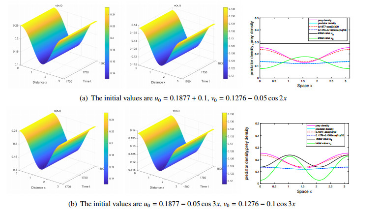
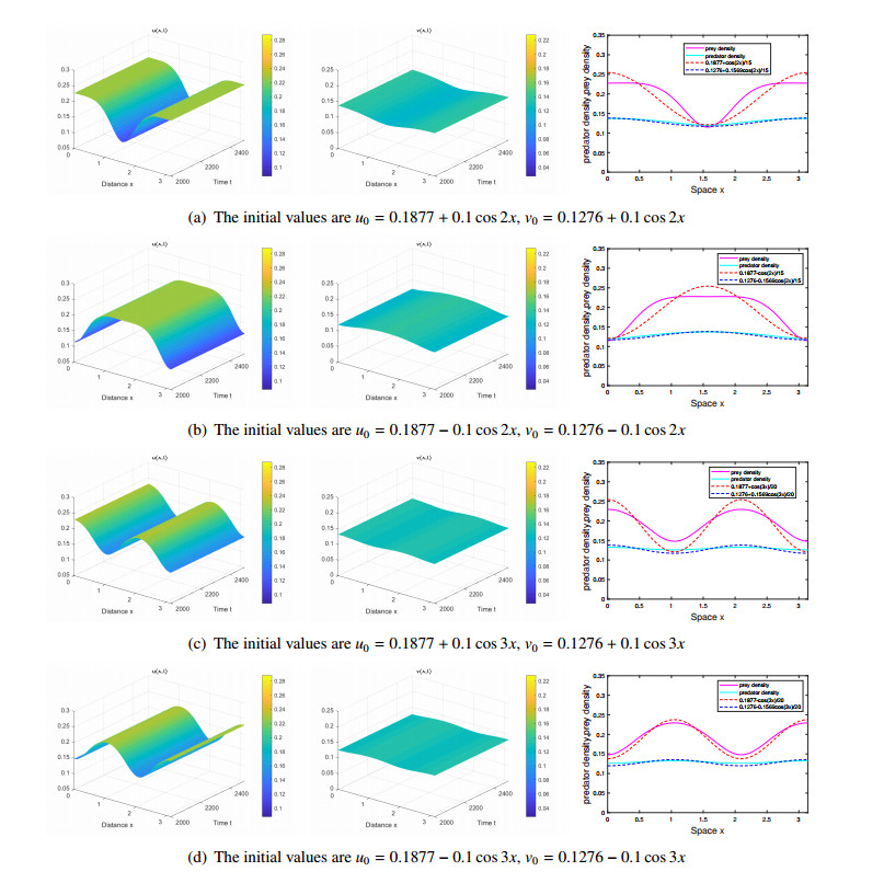
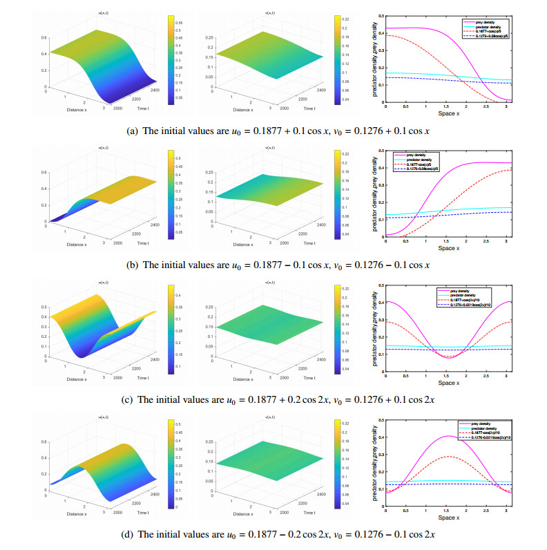
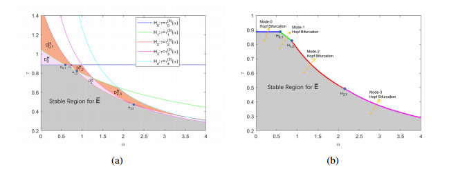
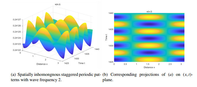
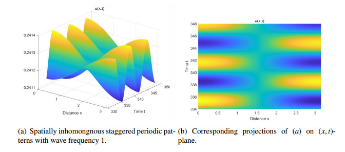
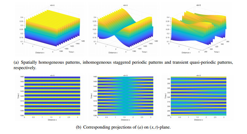
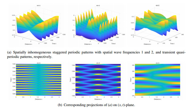
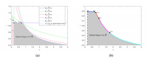
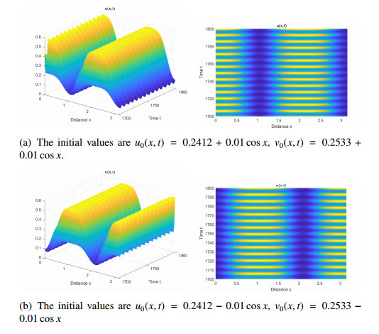
The effects of predator-taxis and conversion time delay on formations of spatiotemporal patterns in a predator-prey model are explored. First, the well-posedness, which implies global existence of classical solutions, is proved. Then, we establish critical conditions for the destabilization of the coexistence equilibrium via Turing/Turing-Turing bifurcations by describing the first Turing bifurcation curve; we also theoretically predict possible bistable/multi-stable spatially heterogeneous patterns. Next, we demonstrate that the coexistence equilibrium can also be destabilized via Hopf, Hopf-Hopf and Turing-Hopf bifurcations; also possible stable/bistable spatially inhomogeneous staggered periodic patterns and bistable spatially inhomogeneous synchronous periodic patterns are theoretically predicted. Finally, numerical experiments also support theoretical predictions and partially extend them. In a word, theoretical analyses indicate that, on the one hand, strong predator-taxis can eliminate spatial patterns caused by self-diffusion; on the other hand, the joint effects of predator-taxis and conversion time delay can induce complex survival patterns, e.g., bistable spatially heterogeneous staggered/synchronous periodic patterns, thus diversifying populations' survival patterns.
Citation: Yue Xing, Weihua Jiang, Xun Cao. Multi-stable and spatiotemporal staggered patterns in a predator-prey model with predator-taxis and delay[J]. Mathematical Biosciences and Engineering, 2023, 20(10): 18413-18444. doi: 10.3934/mbe.2023818
The effects of predator-taxis and conversion time delay on formations of spatiotemporal patterns in a predator-prey model are explored. First, the well-posedness, which implies global existence of classical solutions, is proved. Then, we establish critical conditions for the destabilization of the coexistence equilibrium via Turing/Turing-Turing bifurcations by describing the first Turing bifurcation curve; we also theoretically predict possible bistable/multi-stable spatially heterogeneous patterns. Next, we demonstrate that the coexistence equilibrium can also be destabilized via Hopf, Hopf-Hopf and Turing-Hopf bifurcations; also possible stable/bistable spatially inhomogeneous staggered periodic patterns and bistable spatially inhomogeneous synchronous periodic patterns are theoretically predicted. Finally, numerical experiments also support theoretical predictions and partially extend them. In a word, theoretical analyses indicate that, on the one hand, strong predator-taxis can eliminate spatial patterns caused by self-diffusion; on the other hand, the joint effects of predator-taxis and conversion time delay can induce complex survival patterns, e.g., bistable spatially heterogeneous staggered/synchronous periodic patterns, thus diversifying populations' survival patterns.

| [1] |
S. Guo, Bifurcation and spatio-temporal patterns in a diffusive predator-prey system, Nonlinear Anal. Real World Appl., 42 (2018), 448–477. https://doi.org/10.1016/j.nonrwa.2018.01.011 doi: 10.1016/j.nonrwa.2018.01.011

|
| [2] |
M. Kuwamura, Turing instabilities in prey–predator systems with dormancy of predators, J. Math. Biol., 71 (2015), 125–149. https://doi.org/10.1007/s00285-014-0816-5 doi: 10.1007/s00285-014-0816-5
|
| [3] |
R. Yang, Y. Ding, Spatiotemporal dynamics in a predator-prey model with a functional response increasing in both predator and prey densities, J. Appl. Anal. Comput., 10 (2020), 1962–1979. https://doi.org/10.11948/20190295 doi: 10.11948/20190295
|
| [4] |
J. Huang, S. Ruan, J. Song, Bifurcations in a predator-prey system of Leslie type with generalized Holling type Ⅲ functional response, J. Differ. Equations, 257 (2014), 1721–1752. https://doi.org/10.1016/j.jde.2014.04.024 doi: 10.1016/j.jde.2014.04.024
|
| [5] |
P. Kareiva, A. Mullen, R. Southwood, Population dynamics in spatially complex environments: theory and data, Phil. Trans. R. Soc. Lond. B, 330 (1990), 175–190. https://doi.org/10.1098/rstb.1990.0191 doi: 10.1098/rstb.1990.0191
|
| [6] |
Y. Wang, X. Zhou, W. Jiang, Bifurcations in a diffusive predator-prey system with linear harvesting, Chaos Solitons Fractals, 169 (2023), 1–16. https://doi.org/10.1016/j.chaos.2023.113286 doi: 10.1016/j.chaos.2023.113286
|
| [7] |
W. Xu, H. Shu, Z. Tang, H. Wang, Complex dynamics in a general diffusive predator–prey model with predator maturation delay, J. Dyn. Differ. Equations, 2022 (2022). https://doi.org/10.1007/s10884-022-10176-9 doi: 10.1007/s10884-022-10176-9
|
| [8] | F. S. Berezovskaya, G. P. Karev, Traveling waves in polynomial population models, Dokl. Akad. Nauk, 368 (1999), 318–322. |
| [9] |
E. Keller, L. Segel, Model for chemotaxis, J. Theor. Biol., 30 (1971), 225–234. https://doi.org/10.1016/0022-5193(71)90050-6 doi: 10.1016/0022-5193(71)90050-6
|
| [10] |
A. B. Medvinsky, S. V. Petrovskii, I. A. Tikhonova, H. Malchow, B. L. Li, Spatiotemporal complexity of plankton and fish dynamics, SIAM Rev., 44 (2002), 311–370. https://doi.org/10.1137/S0036144502404442 doi: 10.1137/S0036144502404442
|
| [11] |
J. A. Sherratt, Wavefront propagation in a competition equation with a new motility term modelling contact inhibition between cell populations, R. Soc. Lond. Proc. Ser. A Math. Phys. Eng. Sci., 456 (2000), 2365–2386. https://doi.org/10.1098/rspa.2000.0616 doi: 10.1098/rspa.2000.0616
|
| [12] | E. Curio, The Ethology of Predation, Springer-Verlag, New York, 1976. https://doi.org/10.1007/978-3-642-81028-2 |
| [13] |
M. Hassell, D. Rogers, Insect parasite responses in the development of population models, J. Anim. Ecol., 41 (1972), 661–676. https://doi.org/10.2307/3201 doi: 10.2307/3201
|
| [14] |
M. Hassell, R. May, Stability in insect host-parasitoid models, J. Anim. Ecol., 42 (1973), 693–726. https://doi.org/10.2307/3133 doi: 10.2307/3133
|
| [15] |
W. Murdoch, A. Oaten, Predation and population stability, Adv. Ecol. Res., 9 (1974), 1–131. https://doi.org/10.1016/S0065-2504(08)60288-3 doi: 10.1016/S0065-2504(08)60288-3
|
| [16] |
T. Royama, A comparative study of models for predation and parasitism, Res. Popul. Ecol., 1 (1971), 1–91. https://doi.org/10.1007/BF02511547 doi: 10.1007/BF02511547
|
| [17] |
M. Hassell, R. May, Aggregation in predators and insect parasites and its effect on stability, J. Anim. Ecol., 43 (1974), 567–594. https://doi.org/10.2307/3384 doi: 10.2307/3384
|
| [18] |
P. Kareiva, G. Odell, Swarms of predators exhibit prey taxis if individual predators use area-restricted search, Am. Nat., 130 (1987), 233–270. https://doi.org/10.2307/2461857 doi: 10.2307/2461857
|
| [19] |
C. Cosner, Reaction-diffusion-advection models for the effects and evolution of dispersal, Discrete Contin. Dyn. Syst., 34 (2014), 1701–1745. https://doi.org/10.3934/dcds.2014.34.1701 doi: 10.3934/dcds.2014.34.1701
|
| [20] |
H. Jin, Z. Wang, Global stability of prey-taxis systems, J. Differ. Equations, 262 (2017), 1257–1290. https://doi.org/10.1016/j.jde.2016.10.010 doi: 10.1016/j.jde.2016.10.010
|
| [21] |
C. Liu, S. Guo, Dynamics of a predator–prey system with nonlinear prey-taxis, Nonlinearity, 35 (2022), 4283. https://doi.org/10.1088/1361-6544/ac78bc doi: 10.1088/1361-6544/ac78bc
|
| [22] |
X. Wang, X. Zou, Pattern formation of a predator-prey model with the cost of anti-predator behaviors, Math. Biosci. Eng., 15 (2018), 775–805. https://doi.org/10.3934/mbe.2018035 doi: 10.3934/mbe.2018035
|
| [23] |
S. Wu, J. Wang, J. Shi, Dynamics and pattern formation of a diffusive predator-prey model with predator-taxis, Math. Models Methods Appl. Sci., 28 (2018), 1–36. https://doi.org/10.1142/S0218202518400158 doi: 10.1142/S0218202518400158
|
| [24] |
E. Beretta, Y. Kuang, Global analyses in some delayed ratio-dependent predator-prey systems, Nonlinear Anal., 32 (1998), 381–408. https://doi.org/10.1016/S0362-546X(97)00491-4 doi: 10.1016/S0362-546X(97)00491-4
|
| [25] |
J. Xia, Z. Liu, R. Yuan, S. Ruan, The effects of harvesting and time delay on predator-prey systems with Holling type Ⅱ functional response, SIAM J. Appl. Math., 70 (2009), 1178–1200. https://doi.org/10.1137/080728512 doi: 10.1137/080728512
|
| [26] | Y. Kuang, Delay differential equations with applications in population dynamics, Academic Press, New York, 1993. Available from: https://www.researchgate.net/publication/243764052. |
| [27] |
S. Ruan, On nonlinear dynamics of predator-prey models with discrete delay, Math. Model. Nat. Phenom., 4 (2009), 140–188. https://doi.org/10.1051/mmnp/20094207 doi: 10.1051/mmnp/20094207
|
| [28] |
S. Wu, J. Shi, B. Wu, Global existence of solutions and uniform persistence of a diffusive predator-prey model with prey-taxis, J. Differ. Equations, 260 (2016), 5847–5874. https://doi.org/10.1016/j.jde.2015.12.024 doi: 10.1016/j.jde.2015.12.024
|
| [29] |
J. Wang, S. Wu, J. Shi, Pattern formation in diffusive predator-prey systems with predator-taxis and prey-taxis, Discrete Contin. Dyn. Syst. Ser. B, 26 (2021), 1273. https://doi.org/10.3934/dcdsb.2020162 doi: 10.3934/dcdsb.2020162
|
| [30] |
Q. Cao, J. Wu, Pattern formation of reaction-diffusion system with chemotaxis terms, Chaos, 31 (2021), 113118. https://doi.org/10.1063/5.0054708 doi: 10.1063/5.0054708
|
| [31] |
M. Winkler, Boundedness in the higher-dimensional parabolic-parabolic chemotaxis system with logistic source, Commun. Partial Differ. Equations, 35 (2010), 1516–1537. https://doi.org/10.1080/03605300903473426 doi: 10.1080/03605300903473426
|
| [32] |
T. Xiang, Global dynamics for a diffusive predator-prey model with prey-taxis and classical Lotka-Volterra kinetics, Nonlinear Anal. Real World Appl., 39 (2018), 278–299. https://doi.org/10.1016/j.nonrwa.2017.07.001 doi: 10.1016/j.nonrwa.2017.07.001
|
| [33] |
J. M. Lee, T. Hillen, M. A. Lewis, Pattern formation in prey-taxis systems, J. Biol. Dyn., 3 (2009), 551–573. https://doi.org/10.1080/17513750802716112 doi: 10.1080/17513750802716112
|
| [34] |
J. Gao, S. Guo, Effect of prey-taxis and diffusion on positive steady states for a predator-prey system, Math. Methods. Appl. Sci., 41 (2018), 3570–3587. https://doi.org/10.1002/mma.4847 doi: 10.1002/mma.4847
|
| [35] |
H. Qiu, S. Guo, S. Li, Stability and bifurcation in a predator–prey system with prey-taxis, Int. J. Bifurcation Chaos, 30 (2020), 2050022. https://doi.org/10.1142/S0218127420500224 doi: 10.1142/S0218127420500224
|
| [36] |
X. Gao, Global solution and spatial patterns for a ratio-dependent predator-prey model with predator-taxis, Results Math., 77 (2022), 66. https://doi.org/10.1007/s00025-021-01595-z doi: 10.1007/s00025-021-01595-z
|
| [37] |
Y. Song, Y. Peng, X. Zou, Persistence, stability and Hopf bifurcation in a diffusive ratio-dependent predator-prey model with delay, Int. J. Bifurcation Chaos, 24 (2014), 1450093. https://doi.org/10.1142/S021812741450093X doi: 10.1142/S021812741450093X
|
| [38] |
D. Geng, W. Jiang, Y. Lou, H. Wang, Spatiotemporal patterns in a diffusive predator-prey system with nonlocal intraspecific prey competition, Stud. Appl. Math., 148 (2021), 396–432. https://doi.org/10.1111/sapm.12444 doi: 10.1111/sapm.12444
|
| [39] |
W. Jiang, Q. An, J. Shi, Formulation of the normal form of Turing-Hopf bifurcation in partial functional differential equations, J. Differ. Equations, 268 (2020), 6067–6102. https://doi.org/10.1016/j.jde.2019.11.039 doi: 10.1016/j.jde.2019.11.039
|
| [40] |
J. Shi, C. Wang, H. Wang, Spatial movement with diffusion and memory-based self-diffusion and cross-diffusion, J. Differ. Equations, 305 (2021), 242–269. https://doi.org/10.1016/j.jde.2021.10.021 doi: 10.1016/j.jde.2021.10.021
|
| [41] | M. Wang, Second Order Nonlinear Parabolic Equations, CRC Press, 2021. https://doi.org/10.1201/9781003150169 |
| [42] |
H. Amann, Dynamic theory of quasilinear parabolic equations. Ⅱ. Reaction-diffusion systems, Differ. Integr. Equations, 3 (1990), 13–75. https://doi.org/10.57262/die/1371586185 doi: 10.57262/die/1371586185
|
| [43] |
W. Jiang, H. Wang, X. Cao, Turing instability and Turing-Hopf bifurcation in diffusive Schnakenberg systems with gene expression time delay, J. Dyn. Differ. Equations, 31 (2019), 2223–2247. https://doi.org/10.1007/s10884-018-9702-y doi: 10.1007/s10884-018-9702-y
|
| [44] |
Y. Song, X. Zou, Bifurcation analysis of a diffusive ratio-dependent predator–prey model, Nonlinear Dyn., 78 (2014), 49–70. https://doi.org/10.1007/s11071-014-1421-2 doi: 10.1007/s11071-014-1421-2
|
| [45] |
E. Beretta, Y. Kuang, Geometric stability switch criteria in delay differential systems with delay dependent parameters, SIAM J. Math. Anal., 33 (2002), 1144–1165. https://doi.org/10.1137/S0036141000376086 doi: 10.1137/S0036141000376086
|
| [46] |
F. Yi, E. A. Gaffney, S. S. Lee, The bifurcation analysis of Turing pattern formation induced by delay and diffusion in the Schnakenberg system, Discrete Contin. Dyn. Syst. Ser. B, 22 (2017), 647–668. https://doi.org/10.3934/dcdsb.2017031 doi: 10.3934/dcdsb.2017031
|
| [47] |
X. Jiang, R. Zhang, Z. She, Dynamics of a diffusive predator–prey system with ratio-dependent functional response and time delay, Int. J. Biomath., 13 (2020), 2050036. https://doi.org/10.1142/S1793524520500369 doi: 10.1142/S1793524520500369
|
Figures(14) / Tables(2)

Yue Xing, Weihua Jiang, Xun Cao. Multi-stable and spatiotemporal staggered patterns in a predator-prey model with predator-taxis and delay[J]. Mathematical Biosciences and Engineering, 2023, 20(10): 18413-18444. doi: 10.3934/mbe.2023818


 DownLoad: