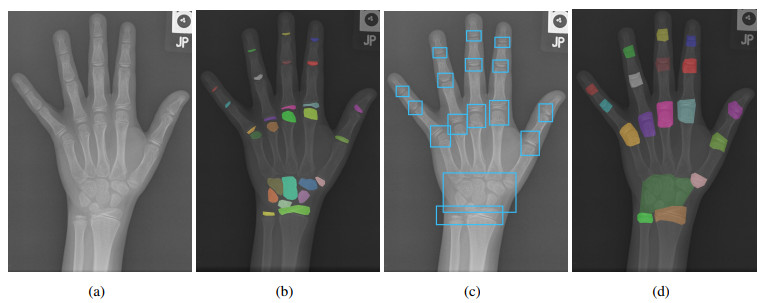
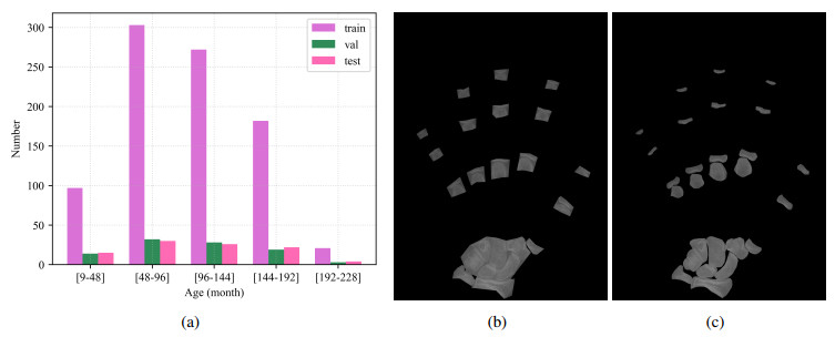
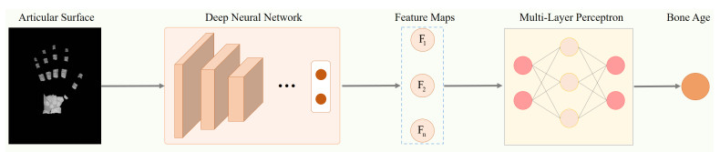
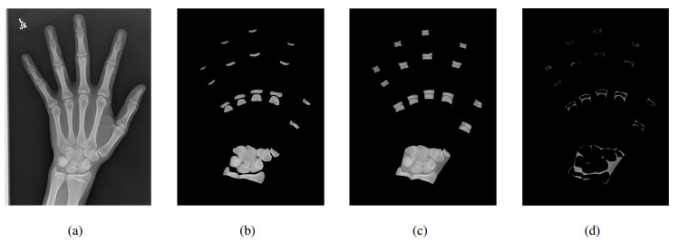
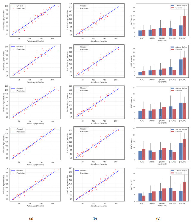
Bone age assessment from articular surface and epiphysis using deep neural networks

Yamei Deng; Yonglu Chen; Qian He; Xu Wang; Yong Liao; Jue Liu; Zhaoran Liu; Jianwei Huang; Ting Song; Yamei Deng; Yonglu Chen; Qian He; Xu Wang; Yong Liao; Jue Liu; Zhaoran Liu; Jianwei Huang; Ting Song

doi:10.3934/mbe.2023585

Mathematical Biosciences and Engineering

2023, Volume 20, Issue 7: 13133-13148. doi: 10.3934/mbe.2023585

Previous Article Next Article

Research article

Bone age assessment from articular surface and epiphysis using deep neural networks

1.
Department of Radiology, Guangdong Provincial Key Laboratory of Major Obstetric Diseases, Guangdong Provincial Clinical Research Center for Obstetrics and Gynecology, The Third Affiliated Hospital of Guangzhou Medical University, Guangzhou 510150, China
2.
School of Automation, Guangdong University of Technology, Guangzhou 510006, China
3.
School of physics, electronics and electrical engineering, Xiangnan University, Chenzhou 423000, China

Academic Editor: Yang Kuang

Received: 28 February 2023 Revised: 18 May 2023 Accepted: 21 May 2023 Published: 06 June 2023

Bone age assessment is of great significance to genetic diagnosis and endocrine diseases. Traditional bone age diagnosis mainly relies on experienced radiologists to examine the regions of interest in hand radiography, but it is time-consuming and may even lead to a vast error between the diagnosis result and the reference. The existing computer-aided methods predict bone age based on general regions of interest but do not explore specific regions of interest in hand radiography. This paper aims to solve such problems by performing bone age prediction on the articular surface and epiphysis from hand radiography using deep convolutional neural networks. The articular surface and epiphysis datasets are established from the Radiological Society of North America (RSNA) pediatric bone age challenge, where the specific feature regions of the articular surface and epiphysis are manually segmented from hand radiography. Five convolutional neural networks, i.e., ResNet50, SENet, DenseNet-121, EfficientNet-b4, and CSPNet, are employed to improve the accuracy and efficiency of bone age diagnosis in clinical applications. Experiments show that the best-performing model can yield a mean absolute error (MAE) of 7.34 months on the proposed articular surface and epiphysis datasets, which is more accurate and fast than the radiologists. The project is available at https://github.com/YameiDeng/BAANet/, and the annotated dataset is also published at https://doi.org/10.5281/zenodo.7947923.
- bone age assessment,
- articular surface,
- epiphysis,
- hand radiography,
- deep neural networks
Citation: Yamei Deng, Yonglu Chen, Qian He, Xu Wang, Yong Liao, Jue Liu, Zhaoran Liu, Jianwei Huang, Ting Song. Bone age assessment from articular surface and epiphysis using deep neural networks[J]. Mathematical Biosciences and Engineering, 2023, 20(7): 13133-13148. doi: 10.3934/mbe.2023585

Related Papers:

Abstract

Bone age assessment is of great significance to genetic diagnosis and endocrine diseases. Traditional bone age diagnosis mainly relies on experienced radiologists to examine the regions of interest in hand radiography, but it is time-consuming and may even lead to a vast error between the diagnosis result and the reference. The existing computer-aided methods predict bone age based on general regions of interest but do not explore specific regions of interest in hand radiography. This paper aims to solve such problems by performing bone age prediction on the articular surface and epiphysis from hand radiography using deep convolutional neural networks. The articular surface and epiphysis datasets are established from the Radiological Society of North America (RSNA) pediatric bone age challenge, where the specific feature regions of the articular surface and epiphysis are manually segmented from hand radiography. Five convolutional neural networks, i.e., ResNet50, SENet, DenseNet-121, EfficientNet-b4, and CSPNet, are employed to improve the accuracy and efficiency of bone age diagnosis in clinical applications. Experiments show that the best-performing model can yield a mean absolute error (MAE) of 7.34 months on the proposed articular surface and epiphysis datasets, which is more accurate and fast than the radiologists. The project is available at https://github.com/YameiDeng/BAANet/, and the annotated dataset is also published at https://doi.org/10.5281/zenodo.7947923.

References

[1]	P. Hao, S. Chokuwa, X. Xie, F. Wu, J. Wu, C. Bai, Skeletal bone age assessments for young children based on regression convolutional neural networks, Math. Biosci. Eng., 16 (2019), 6454–6466.
[2]	W. Lin, F. Yang, Computational analysis of cutting parameters based on gradient voronoi model of cancellous bone, Math. Biosci. Eng., 19 (2022), 11657–11674. https://doi.org/10.3934/mbe.2022542 doi: 10.3934/mbe.2022542
[3]	S. L Truesdell, M. M Saunders, Bone remodeling platforms: Understanding the need for multicellular lab-on-a-chip systems and predictive agent-based models, Math. Biosci. Eng., 17 (2020).
[4]	A. Nordenstrom, H. Falhammar, Management of endocrine disease: Diagnosis and management of the patient with non-classic CAH due to 21-hydroxylase deficiency, Eur. J. Endocrinol., 180 (2019), R127–R145.
[5]	A. C. Morani, C. T. Jensen, M. A. Habra, M. M. Agrons, C. O. Menias, N. A. Wagner-Bartak, et al., Adrenocortical hyperplasia: a review of clinical presentation and imaging, Abdominal Radiol., 45 (2020), 917–927. https://doi.org/10.1007/s00261-019-02048-6 doi: 10.1007/s00261-019-02048-6
[6]	J.-C. Carel, J. Léger, Precocious puberty, New England J. Med., 358 (2008), 2366–2377. https://doi.org/10.1056/NEJMcp0800459 doi: 10.1056/NEJMcp0800459
[7]	K. Kyostila, J. E. Niskanen, M. Arumilli, J. Donner, M. K. Hytönen, H. Lohi, Intronic variant in POU1F1 associated with canine pituitary dwarfism, Human Gene., 140 (2021), 1553–1562. https://doi.org/10.1007/s00439-021-02259-2 doi: 10.1007/s00439-021-02259-2
[8]	K. C. Lee, K. H. Lee, C. H. Kang, K. S. Ahn, L. Y. Chung, J. J. Lee, et al., Clinical validation of a deep learning-based hybrid (Greulich-Pyle and modified Tanner-Whitehouse) method for bone age assessment, Korean J. Radiol., 22 (2021), 2017–2025. https://doi.org/10.3348/kjr.2020.1468 doi: 10.3348/kjr.2020.1468
[9]	P. Lv, C. Zhang, Tanner–Whitehouse skeletal maturity score derived from ultrasound images to evaluate bone age, Eur. Radiol., 2022 (2022), 1–8.
[10]	S. Zhang, L. Liu, The skeletal development standards of hand and wrist for Chinese Children¡ªChina 05 I. TW_3-C RUS, TW_3-C Carpal, and RUS-CHN methods, Chin. J. Sports Med., 2023 (2023), 6–13.
[11]	J. R. Kim, Y. S. Lee, J. Yu, Assessment of bone age in prepubertal healthy Korean children: comparison among the Korean standard bone age chart, Greulich-Pyle method, and Tanner-Whitehouse method, Korean J. Radiol., 16 (2015), 201–205. https://doi.org/10.3348/kjr.2015.16.1.201 doi: 10.3348/kjr.2015.16.1.201
[12]	C. Gao, Q. Qian, Y. Li, X. Xing, X. He, M. Lin, et al., A comparative study of three bone age assessment methods on Chinese preschool-aged children, Front. Pediatr., 10 (2022), 1–12. https://doi.org/10.3389/fped.2022.976565 doi: 10.3389/fped.2022.976565
[13]	H. Liu, M. Liu, D. Li, W. Zheng, L. Yin, R. Wang, Recent advances in pulse-coupled neural networks with applications in image processing, Electronics, 11 (2022), 3264. https://doi.org/10.3390/electronics11203264 doi: 10.3390/electronics11203264
[14]	Y. Ban, Y. Wang, S. Liu, B. Yang, M. Liu, L. Yin, et al., 2d/3d multimode medical image alignment based on spatial histograms, Appl. Sci., 12 (2022), 8261. https://doi.org/10.3390/app12168261 doi: 10.3390/app12168261
[15]	S. Xiong, B. Li, S. Zhu, DCGNN: A single-stage 3D object detection network based on density clustering and graph neural network, Complex Intell. Syst., 2022 (2022), 1–10.
[16]	C. Spampinato, S. Palazzo, D. Giordano, M. Aldinucci, R. Leonardi, Deep learning for automated skeletal bone age assessment in X-ray images, Med. Image Anal., 36 (2017), 41–51. https://doi.org/10.1016/j.media.2016.10.010 doi: 10.1016/j.media.2016.10.010
[17]	D. B. Larson, M. C. Chen, M. P. Lungren, S. S. Halabi, N. V. Stence, C. P. Langlotz, Performance of a deep-learning neural network model in assessing skeletal maturity on pediatric hand radiographs, Radiology, 287 (2018), 313–322. https://doi.org/10.1148/radiol.2017170236 doi: 10.1148/radiol.2017170236
[18]	Y. Liu, C. Zhang, J. Cheng, X. Chen, Z. J. Wang, A multi-scale data fusion framework for bone age assessment with convolutional neural networks, Comput. Biol. Med., 108 (2019), 161–173. https://doi.org/10.1016/j.compbiomed.2019.03.015 doi: 10.1016/j.compbiomed.2019.03.015
[19]	Q. H. Nguyen, B. P. Nguyen, M. T. Nguyen, M. C. Chua, T. T. Do, N. Nghiem, Bone age assessment and sex determination using transfer learning, Expert Syst. Appl., 200 (2022), 116926. https://doi.org/10.1016/j.eswa.2022.116926 doi: 10.1016/j.eswa.2022.116926
[20]	X. Ren, T. Li, X. Yang, S. Wang, S. Ahmad, L. Xiang, et al., Regression convolutional neural network for automated pediatric bone age assessment from hand radiograph, IEEE J. Biomed. Health Inf., 23 (2018), 2030–2038. https://doi.org/10.1109/JBHI.2018.2876916 doi: 10.1109/JBHI.2018.2876916
[21]	C. Liu, H. Xie, Y. Zhang, Self-supervised attention mechanism for pediatric bone age assessment with efficient weak annotation, IEEE Trans. Med. Imaging, 40 (2020), 2685–2697. https://doi.org/10.1109/TMI.2020.3046672 doi: 10.1109/TMI.2020.3046672
[22]	N. E. Reddy, J. C. Rayan, A. V. Annapragada, N. F. Mahmood, A. E. Scheslinger, W. Zhang, et al., Bone age determination using only the index finger: a novel approach using a convolutional neural network compared with human radiologists, Pediatr. Radiol., 50 (2020), 516–523. https://doi.org/10.1007/s00247-019-04587-y doi: 10.1007/s00247-019-04587-y
[23]	S. Mutasa, P. D. Chang, C. Ruzal-Shapiro, R. Ayyala, MABAL: A novel deep-learning architecture for machine-assisted bone age labeling, J. Dig. Imaging, 31 (2018), 513–519. https://doi.org/10.1007/s10278-018-0053-3 doi: 10.1007/s10278-018-0053-3
[24]	X. Li, Y. Jiang, Y. Liu, J. Zhang, S. Yin, H. Luo, RAGCN: Region aggregation graph convolutional network for bone age assessment from X-ray images, IEEE Trans. Instru. Measure., 71 (2022), 1–12.
[25]	S. S. Halabi, L. M. Prevedello, J. Kalpathy-Cramer, A. B. Mamonov, A. Bilbily, M. Cicero, et al., The RSNA pediatric bone age machine learning challenge, Radiology, 290 (2019), 498–503. https://doi.org/10.1148/radiol.2018180736 doi: 10.1148/radiol.2018180736
[26]	B. C. Russell, A. Torralba, K. P. Murphy, W. T. Freeman, LabelMe: a database and web-based tool for image annotation, Int. J. Comput. Vision, 77 (2008), 157–173. https://doi.org/10.1007/s11263-007-0090-8 doi: 10.1007/s11263-007-0090-8
[27]	K. He, X. Zhang, S. Ren, J. Sun, Deep residual learning for image recognition, in Proceedings of the IEEE Conference on Computer Vision and Pattern Recognition (CVPR), 2016,770–778.
[28]	J. Hu, L. Shen, G. Sun, Squeeze-and-excitation networks, in Proceedings of the IEEE conference on computer vision and pattern recognition (CVPR), 2018, 7132–7141.
[29]	G. Huang, Z. Liu, L. Van Der Maaten, K. Q. Weinberger, Densely connected convolutional networks, in Proceedings of the IEEE conference on computer vision and pattern recognition (CVPR), 2017, 4700–4708.
[30]	M. Tan, Q. Le, Efficientnet: Rethinking model scaling for convolutional neural networks, in Proceedings of the International conference on machine learning (ICLR), 2019, 6105–6114.
[31]	C. Y. Wang, H. Y. M. Liao, Y. H. Wu, P. Y. Chen, J. W. Hsieh, I. H. Yeh, CSPNet: A new backbone that can enhance learning capability of CNN, in Proceedings of the IEEE/CVF conference on computer vision and pattern recognition workshops (CVPR), 2020,390–391.
[32]	D. Giordano, C. Spampinato, G. Scarciofalo, R. Leonardi, An automatic system for skeletal bone age measurement by robust processing of carpal and epiphysial/metaphysial bones, IEEE Trans. Instru. Measure., 59 (2010), 2539–2553. https://doi.org/10.1109/TIM.2010.2058210 doi: 10.1109/TIM.2010.2058210
[33]	D. Knapik, J. Sanders, A. Gilmore, D. Weber, D. Cooperman, R. Liu, A quantitative method for the radiological assessment of skeletal maturity using the distal femur, Bone Joint J., 100 (2018), 1106–1111.
[34]	A. K. Bhat, A. M. Acharya, M. Pai, Radiology of the wrist and hand, in Clinical Examination of the Hand, CRC Press, (2022), 275–299.
[35]	K. S. Ahn, B. Bae, W. Y. Jang, J. H. Lee, J. H. Lee, S. Oh, B. H. Kim, et al., Assessment of rapidly advancing bone age during puberty on elbow radiographs using a deep neural network model, Eur. Radiol., 31 (2021), 8947–8955. https://doi.org/10.1007/s00330-021-08096-1 doi: 10.1007/s00330-021-08096-1
[36]	U. Nemec, S. F. Nemec, M. Weber, et al., Human long bone development in vivo: analysis of the distal femoral epimetaphysis on MR images of fetuses, Radiology, 267 (2013), 570–580. https://doi.org/10.1148/radiol.13112441 doi: 10.1148/radiol.13112441
[37]	A. Vaswani, N. Shazeer, N. Parmar, J. Uszkoreit, L. Jones, A. N. Gomez, et al., Attention is all you need, in Proceedings of the 31st International Conference on Neural Information Processing Systems (NIPS), 2017, 5998–6008.
[38]	Z. Q. Zhao, P. Zheng, S. Xu, X. Wu, Object detection with deep learning: A review, IEEE Trans. Neural Networks Learn. syst., 30 (2019), 3212–3232. https://doi.org/10.1109/TNNLS.2018.2876865 doi: 10.1109/TNNLS.2018.2876865
[39]	S. Ren, K. He, R. Girshick, J. Sun, Faster R-CNN: Towards real-time object detection with region proposal networks, IEEE Trans. Pattern Anal. Mach. Intell., 39 (2017), 1137–1149. https://doi.org/10.1109/TPAMI.2016.2577031 doi: 10.1109/TPAMI.2016.2577031
[40]	A. Dosovitskiy, L. Beyer, A. Kolesnikov, D. Weissenborn, X. Zhai, T. Unterthiner, et al., An image is worth 16x16 words: Transformers for image recognition at scale, in Proceedings of the International Conference on Learning Representations (ICLR), 2020, 1–21.
[41]	M. Roberts, D. Driggs, M. Thorpe, J. Gilbey, M. Yeung, S. Ursprung, et al., Common pitfalls and recommendations for using machine learning to detect and prognosticate for COVID-19 using chest radiographs and CT scans, Nat. Mach. Intell., 3 (2021), 199–217.
[42]	Z. Liu, Y. Lin, Y. Cao, H. Hu, Y. Wei, Z. Zhang, et al., Swin transformer: Hierarchical vision transformer using shifted windows, in Proceedings of the IEEE/CVF international conference on computer vision (CVPR), 2021 (2021), 10012–10022.
[43]	C. Y. Wang, A. Bochkovskiy, H. Y. M. Liao, Scaled-yolov4: Scaling cross stage partial network, in Proceedings of the IEEE/cvf conference on computer vision and pattern recognition (CVPR), (2021), 13029–13038.
[44]	A. Paszke, S. Gross, F. Massa, A. Lerer, J. Bradbury, G. Chanan, et al., Pytorch: An imperative style, high-performance deep learning library, in Proceedings of the Advances in Neural Information Processing Systems (NIPS), (2019), 8026–8037.
[45]	L. Bottou, F. E. Curtis, J. Nocedal, Optimization methods for large-scale machine learning, Siam Rev., 60 (2018), 223–311. https://doi.org/10.1137/16M1080173 doi: 10.1137/16M1080173
[46]	C. Gonzalez, M. Escobar, L. Daza, F. Torres, G. Triana, P. Arbelaez, SIMBA: Specific identity markers for bone age assessment, in Proceeding of Medical Image Computing and Computer Assisted Intervention (MICCAI), (2020), 753–763.
[47]	C. Chen, Z. Chen, X. Jin, L. Li, W. Speier, C. W. Arnold, Attention-guided discriminative region localization and label distribution learning for bone age assessment, IEEE J. Biomed. Health Inf., 26 (2021), 1208–1218.
[48]	B. D. Lee, M. S. Lee, Automated bone age assessment using artificial intelligence: the future of bone age assessment, Korean J. Radiol., 22 (2021), 792–800. https://doi.org/10.3348/kjr.2020.0941 doi: 10.3348/kjr.2020.0941

Reader Comments

Your name:*

Email:*
© 2023 the Author(s), licensee AIMS Press. This is an open access article distributed under the terms of the Creative Commons Attribution License (http://creativecommons.org/licenses/by/4.0)