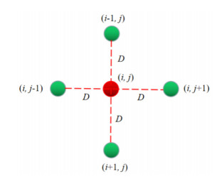
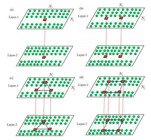
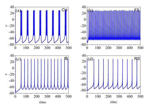
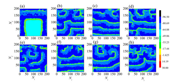
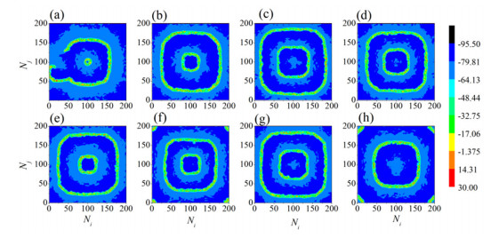
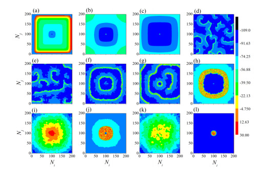
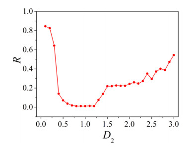
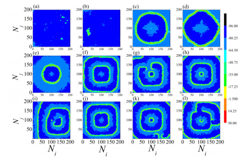
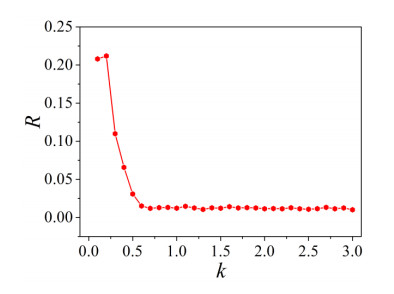
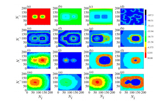
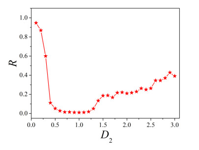
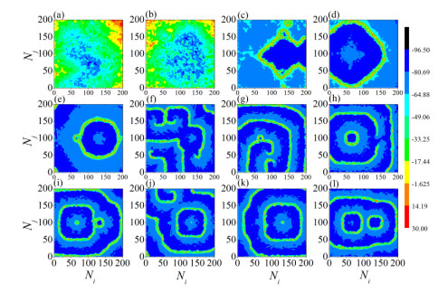
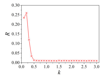
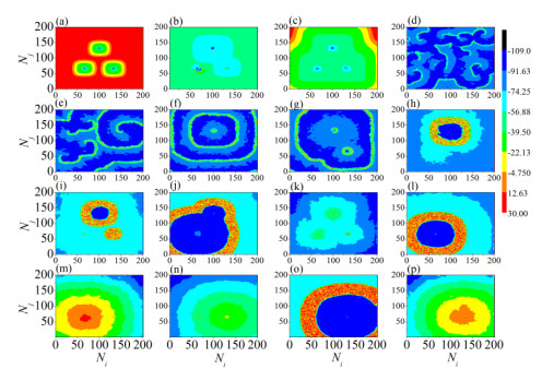
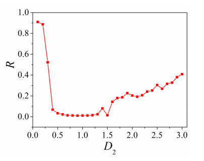
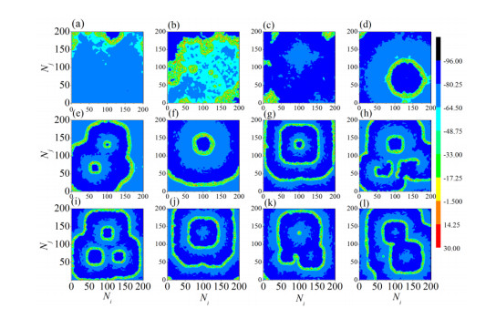
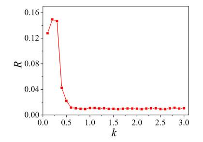
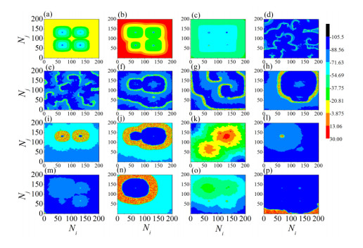
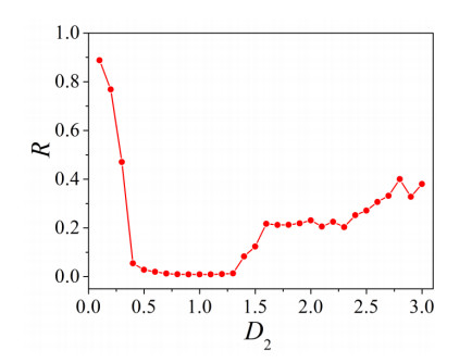
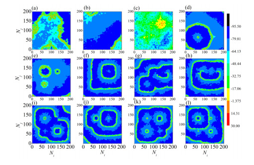
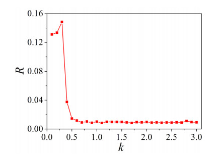
The firing behavior and bifurcation of different types of Izhikevich neurons are analyzed firstly through numerical simulation. Then, a bi-layer neural network driven by random boundary is constructed by means of system simulation, in which each layer is a matrix network composed of 200 × 200 Izhikevich neurons, and the bi-layer neural network is connected by multi-area channels. Finally, the emergence and disappearance of spiral wave in matrix neural network are investigated, and the synchronization property of neural network is discussed. Obtained results show that random boundary can induce spiral waves under appropriate conditions, and it is clear that the emergence and disappearance of spiral wave can be observed only when the matrix neural network is constructed by regular spiking Izhikevich neurons, while it cannot be observed in neural networks constructed by other modes such as fast spiking, chattering and intrinsically bursting. Further research shows that the variation of synchronization factor with coupling strength between adjacent neurons shows an inverse bell-like curve in the form of "inverse stochastic resonance", but the variation of synchronization factor with coupling strength of inter-layer channels is a curve that is approximately monotonically decreasing. More importantly, it is found that lower synchronicity is helpful to develop spatiotemporal patterns. These results enable people to further understand the collective dynamics of neural networks under random conditions.
Citation: Guowei Wang, Yan Fu. Spatiotemporal patterns and collective dynamics of bi-layer coupled Izhikevich neural networks with multi-area channels[J]. Mathematical Biosciences and Engineering, 2023, 20(2): 3944-3969. doi: 10.3934/mbe.2023184
The firing behavior and bifurcation of different types of Izhikevich neurons are analyzed firstly through numerical simulation. Then, a bi-layer neural network driven by random boundary is constructed by means of system simulation, in which each layer is a matrix network composed of 200 × 200 Izhikevich neurons, and the bi-layer neural network is connected by multi-area channels. Finally, the emergence and disappearance of spiral wave in matrix neural network are investigated, and the synchronization property of neural network is discussed. Obtained results show that random boundary can induce spiral waves under appropriate conditions, and it is clear that the emergence and disappearance of spiral wave can be observed only when the matrix neural network is constructed by regular spiking Izhikevich neurons, while it cannot be observed in neural networks constructed by other modes such as fast spiking, chattering and intrinsically bursting. Further research shows that the variation of synchronization factor with coupling strength between adjacent neurons shows an inverse bell-like curve in the form of "inverse stochastic resonance", but the variation of synchronization factor with coupling strength of inter-layer channels is a curve that is approximately monotonically decreasing. More importantly, it is found that lower synchronicity is helpful to develop spatiotemporal patterns. These results enable people to further understand the collective dynamics of neural networks under random conditions.

| [1] |
V. S. Zykov, Spiral wave initiation in excitable media, Philos. Trans. R. Soc. A, 376 (2018), 20170379. https://doi.org/10.1098/rsta.2017.0379 doi: 10.1098/rsta.2017.0379

|
| [2] |
F. Amdjadi, A numerical method for the dynamics and stability of spiral waves, Appl. Math. Comput., 217 (2010), 3385–3391. https://doi.org/10.1016/j.amc.2010.09.002 doi: 10.1016/j.amc.2010.09.002
|
| [3] |
A. Bukh, G. Strelkova, V. Anishchenko, Spiral wave patterns in a two-dimensional lattice of nonlocally coupled maps modeling neural activity, Chaos Solitons Fractals, 120 (2019), 75–82. https://doi.org/10.1016/j.chaos.2018.11.037 doi: 10.1016/j.chaos.2018.11.037
|
| [4] |
A. V. Bukh, E. Schöll, V. S. Anishchenko, Synchronization of spiral wave patterns in two-layer 2D lattices of nonlocally coupled discrete oscillators, Chaos, 29 (2019), 053105. https://doi.org/10.1063/1.5092352 doi: 10.1063/1.5092352
|
| [5] |
A. V. Bukh, V. S. Anishchenko, Spiral, target, and chimera wave structures in a two- dimensional ensemble of nonlocally coupled van der Pol oscillators, Tech. Phys. Lett., 45 (2019), 675–678. https://doi.org/10.1134/S1063785019070046 doi: 10.1134/S1063785019070046
|
| [6] |
E. M. Cherry, F. H. Fenton, Visualization of spiral and scroll waves in simulated and experimental cardiac tissue, New J. Phys., 10 (2008), 125016. https://doi.org/10.1088/1367-2630/10/12/125016 doi: 10.1088/1367-2630/10/12/125016
|
| [7] |
X. Cui, X. Huang, Z. Di, Target wave imagery in nonlinear oscillatory systems, Europhys. Lett., 112 (2015), 54003. https://doi.org/10.1209/0295-5075/112/54003 doi: 10.1209/0295-5075/112/54003
|
| [8] |
B. W. Li, X. Gao, Z. G. Deng, H. P. Ying, H. Zhang, Circular-interface selected wave patterns in the complex Ginzburg-Landau equation, Europhys. Lett., 91 (2010), 34001. https://doi.org/10.1209/0295-5075/91/34001 doi: 10.1209/0295-5075/91/34001
|
| [9] |
R. Wang, J. Li, M. Du, J. Lei, Y. Wu, Transition of spatiotemporal patterns in neuronal networks with chemical synapses, Commun. Nonlinear Sci. Numer. Simul., 40 (2016), 80–88. https://doi.org/10.1016/j.cnsns.2016.04.018 doi: 10.1016/j.cnsns.2016.04.018
|
| [10] |
M. Y. Ge, G. W. Wang, Y. Jia, Influence of the Gaussian colored noise and electromagnetic radiation on the propagation of subthreshold signals in feedforward neural networks, Sci. China Technol. Sci., 64 (2021), 847–857. https://doi.org/10.1007/s11431-020-1696-8 doi: 10.1007/s11431-020-1696-8
|
| [11] |
A. V. Bukh, V. S. Anishchenko, Features of the synchronization of spiral wave structures in interacting lattices of nonlocally coupled maps, Russ. J. Nonlinear Dyn., 16 (2020), 243–257. https://doi.org/10.20537/nd200202 doi: 10.20537/nd200202
|
| [12] |
M. C. Cai, J. T. Pan, H. Zhang, Electric-field-sustained spiral waves in subexcitable media, Phys. Rev. E, 86 (2012), 016208. https://doi.org/10.1103/PhysRevE.86.016208 doi: 10.1103/PhysRevE.86.016208
|
| [13] | J. X. Chen, J. R. Xu, H. P. Ying, Resonant drift of spiral waves induced by mechanical deformation, Int. J. Mod. Phys. B, 2 4(2012), 5733–5741. https://doi.org/10.1142/S0217979210056323 |
| [14] |
J. Chen, L. Peng, Y. Zhao, S. You, N. Wu, H. Ying, et al., Dynamics of spiral waves driven by a rotating electric field, Commun. Nonlinear Sci. Numer. Simul., 19 (2014), 60–66. https://doi.org/10.1016/j.cnsns.2013.03.010 doi: 10.1016/j.cnsns.2013.03.010
|
| [15] |
C. N. Wang, J. Ma, B. Hu, W. Jin, Formation of multi-armed spiral waves in neuronal network induced by adjusting ion channel conductance, Int. J. Mod. Phys. B, 29 (2015), 1550043. https://doi.org/10.1142/S0217979215500435 doi: 10.1142/S0217979215500435
|
| [16] |
J. Gao, Q. Wang, H. Lv, Super-spiral structures of bi-stable spiral waves and a new instability of spiral waves, Chem. Phys. Lett., 685 (2017), 205–209. https://doi.org/10.1016/j.cplett.2017.07.061 doi: 10.1016/j.cplett.2017.07.061
|
| [17] |
J. Z. Gao, S. X. Yang, L. L. Xie, J. H. Gao, Synchronizing spiral waves in a coupled Rössler system, Chin. Phys. B, 20 (2011), 030505. https://doi.org/10.1088/1674-1056/20/3/030505 doi: 10.1088/1674-1056/20/3/030505
|
| [18] |
Y. Nishitani, C. Hosokawa, Y. Mizuno-Matsumoto, T. Miyoshi, S. Tamura, Classification of spike wave propagations in a cultured neuronal network: Investigating a brain communication mechanism, AIMS Neurosci., 4 (2017), 1–13. https://doi.org/10.3934/Neuroscience.2017.1.1 doi: 10.3934/Neuroscience.2017.1.1
|
| [19] |
J. Ma, Y. Xu, J. Tang, C. Wang, Defects formation and wave emitting from defects in excitable media, Commun. Nonlinear Sci. Numer. Simul., 34 (2016), 55–65. https://doi.org/10.1016/j.cnsns.2015.10.013 doi: 10.1016/j.cnsns.2015.10.013
|
| [20] |
R. Sirovich, L. Sacerdote, A. E. P. Villa, Cooperative behavior in a jump diffusion model for a simple network of spiking neurons, Math. Biosci. Eng., 11 (2014), 385–401. https://doi.org/10.3934/mbe.2014.11.385 doi: 10.3934/mbe.2014.11.385
|
| [21] |
A. Gholami, O. Steinbock, V. Zykov, E. Bodenschatz, Flow-driven instabilities during pattern formation of Dictyostelium discoideum, New J. Phys., 17 (2015), 063007. https://doi.org/10.1088/1367-2630/17/6/063007 doi: 10.1088/1367-2630/17/6/063007
|
| [22] |
S. Gong, X. Tang, J. Zheng, M. A. Nascimento, H. Varela, Y. Zhao, et al., Amplitude-modulated spiral waves arising from a secondary Hopf bifurcation in mixed-mode oscillatory media, Chem. Phys. Lett., 567 (2013), 55–59. https://doi.org/10.1016/j.cplett.2013.02.042 doi: 10.1016/j.cplett.2013.02.042
|
| [23] |
S. Blankenburg, B. Lindner, The effect of positive interspike interval correlations on neuronal information transmission, Math. Biosci. Eng., 13 (2016), 461–481. https://doi.org/10.3934/mbe.2016001 doi: 10.3934/mbe.2016001
|
| [24] | E. Griv, I. G. Jiang, D. Russeil, Parameters of the galactic density-wave spiral structure, line-of-sight velocities of 156 star-forming regions, New Astronomy, 35 (2015), 40–47. https://doi.org/10.1016/j.newast.2014.09.001 |
| [25] |
H. G. Gu, B. Jia, Y. Y. Li, G. R. Chen, White noise-induced spiral waves and multiple spatial coherence resonances in a neuronal network with type I excitability, Phys. A, 392 (2013), 1361–1374. https://doi.org/10.1016/j.physa.2012.11.049 doi: 10.1016/j.physa.2012.11.049
|
| [26] |
S. Guo, Q. Dai, H. Cheng, H. Li, F. Xie, J. Yang, Spiral wave chimera in two-dimensional nonlocally coupled Fitzhugh-Nagumo systems, Chaos Solitons Fractals, 114 (2018), 394–399. https://doi.org/10.1016/j.chaos.2018.07.029 doi: 10.1016/j.chaos.2018.07.029
|
| [27] |
J. Ma, J. Tang, C. N. Wang, Y. Jia, Propagation and synchronization of Ca2+ spiral waves in excitable media, Int. J. Bifurcation Chaos, 21 (2011), 587–601. https://doi.org/10.1142/S0218127411028635 doi: 10.1142/S0218127411028635
|
| [28] |
C. Hall, D. Forgan, K. Rice, T. J. Harries, P. D. Klaassen, B. Biller, Directly observing continuum emission from self-gravitating spiral waves, Mon. Not. R. Astron. Soc., 458 (2016), 306–318. https://doi.org/10.1093/mnras/stw296 doi: 10.1093/mnras/stw296
|
| [29] |
L. H. Zhao, S. Wen, M. Xu, K. Shi, S. Zhu, T. Huang, PID control for output synchronization of multiple output coupled complex networks, IEEE Trans. Network Sci. Eng., 9 (2022), 1553–1566. https://doi.org/10.1109/TNSE.2022.3147786 doi: 10.1109/TNSE.2022.3147786
|
| [30] | L. H. Zhao, S. Wen, C. Li, K. Shi, T. Huang, A recent survey on control for synchronization and passivity of complex networks, IEEE Trans. Network Sci. Eng., 9 (2022), 4235–4254. https://doi.org/10.1109/TNSE.2022.3196786 |
| [31] |
G. Hu, X. Li, S. Lu, Y. Wang, Bifurcation analysis and spatiotemporal patterns in a diffusive predator-prey model, Int. J. Bifurcation Chaos, 24 (2014), 1450081. https://doi.org/10.1142/S0218127414500813 doi: 10.1142/S0218127414500813
|
| [32] |
H. Hu, X. Li, Fang, X. Fu, L. Ji, Q. Li, Inducing and modulating spiral waves by delayed feedback in a uniform oscillatory reaction-diffusion system, Chem. Phys., 371 (2010), 60–65. https://doi.org/10.1016/j.chemphys.2010.04.004 doi: 10.1016/j.chemphys.2010.04.004
|
| [33] |
M. Montesinos, S. Perez, S. Casassus, S. Marino, J. Cuadra, V. Christiaens, Spiral waves triggered by shadows in transition disks, Astrophys. J. Lett., 823 (2016), L8. https://doi.org/10.3847/2041-8205/823/1/L8 doi: 10.3847/2041-8205/823/1/L8
|
| [34] |
C. Huang, X. Cui, Z. Di, Competition of spiral waves in heterogeneous CGLE systems, Nonlinear Dyn., 98 (2019), 561–571. https://doi.org/10.1007/s11071-019-05212-1 doi: 10.1007/s11071-019-05212-1
|
| [35] |
X. Huang, W. Xu, J. Liang, K. Takagaki, X. Gao, J. Wu, Spiral wave dynamics in neocortex, Neuron, 68 (2010), 978–990. https://doi.org/10.1016/j.neuron.2010.11.007 doi: 10.1016/j.neuron.2010.11.007
|
| [36] |
I. A. Shepelev, S. S. Muni, T. E. Vadivasova, Synchronization of wave structures in a heterogeneous multiplex network of 2D lattices with attractive and repulsive intra-layer coupling, Chaos, 31 (2021), 021104. https://doi.org/10.1063/5.0044327 doi: 10.1063/5.0044327
|
| [37] |
S. Jacquir, S. Binczak, B. Xu, G. Laurent, D. Vandroux, P. Athias, et al., Investigation of micro spiral waves at cellular level using a microelectrode arrays technology, Int. J. Bifurcation Chaos, 21 (2011), 209–223. https://doi.org/10.1142/S0218127411028374 doi: 10.1142/S0218127411028374
|
| [38] |
D. Jaiswal, J. C. Kalita, Novel high-order compact approach for dynamics of spiral waves in excitable media, Appl. Math. Modell., 77 (2020), 341–359. https://doi.org/10.1016/j.apm.2019.07.029 doi: 10.1016/j.apm.2019.07.029
|
| [39] |
A. R. Nayak, R. Pandit, Spiral-wave dynamics in ionically realistic mathematical models for human ventricular tissue: the effects of periodic deformation, Front. Physiol., 5 (2014), 207–225. https://doi.org/10.3389/fphys.2014.00207 doi: 10.3389/fphys.2014.00207
|
| [40] |
V. N. Kachalov, N. N. Kudryashova, K. I. Agladze, Spontaneous spiral wave breakup caused by pinning to the tissue defect, JETP Lett., 104 (2016), 635–638. https://doi.org/10.1134/S0021364016210025 doi: 10.1134/S0021364016210025
|
| [41] | N. V. Kandaurova, V. S. Chekanov, V. V. Chekanov, Observation of the autowave process in the near-electrode layer of the magnetic fluid, Spiral waves formation mechanism, J. Mol. Liq., 272 (2018), 828–833. https://doi.org/10.1016/j.molliq.2018.10.073 |
| [42] |
C. Gu, P. Wang, T. Weng, H. Yang, J. Rohling Heterogeneity of neuronal properties determines the collective behavior of the neurons in the suprachiasmatic nucleus, Math. Biosci. Eng., 16 (2019), 1893–1913. https://doi.org/10.3934/mbe.2019092 doi: 10.3934/mbe.2019092
|
| [43] |
F. M. G. Magpantay, X. Zou, Wave fronts in neuronal fields with nonlocal post-synaptic axonal connections and delayed nonlocal feedback connections, Math. Biosci. Eng., 7 (2010), 421–442. https://doi.org/10.3934/mbe.2010.7.421 doi: 10.3934/mbe.2010.7.421
|
| [44] |
S. Kawaguchi, Propagating wave segment under global feedback, Eur. Phys. J. B., 87 (2014), 1–10. https://doi.org/10.1140/epjb/e2014-40999-1 doi: 10.1140/epjb/e2014-40999-1
|
| [45] |
T. Y. Li, G. W. Wang, D. Yu, Q. Ding, Y. Jia, Synchronization mode transitions induced by chaos in modified Morris-Lecar neural systems with weak coupling, Nonlinear Dyn., 108 (2022), 2611–2625. https://doi.org/10.1007/s11071-022-07318-5 doi: 10.1007/s11071-022-07318-5
|
| [46] |
M. Mehrabbeik, F. Parastesh, J. Ramadoss, K. Rajagopal, H. Namazi, S. Jafari, Synchronization and chimera states in the network of electrochemically coupled memristive Rulkov neuron maps, Math. Biosci. Eng., 18 (2021), 9394–9409. https://doi.org/10.3934/mbe.2021462 doi: 10.3934/mbe.2021462
|
| [47] | N. E. Kouvaris, S. Hata, A. D. Guilera, Pattern formation in multiplex networks, Sci. Rep. 5 (2015), 1–9. https://doi.org/10.1038/srep10840 |
| [48] |
P. Kuklik, P. Sanders, L. Szumowski, J. J. Żebrowski, Attraction and repulsion of spiral waves by inhomogeneity of conduction anisotropy—a model of spiral wave interaction with electrical remodeling of heart tissue, J. Biol. Phys., 39 (2013), 67–80. https://doi.org/10.1007/s10867-012-9286-4 doi: 10.1007/s10867-012-9286-4
|
| [49] | P. Kuklik, L. Szumowski, P. Sanders, J. J. Żebrowski, Spiral wave breakup in excitable media with an inhomogeneity of conduction anisotropy, Comput. Biol. Med., 40 (99), 775–780. https://doi.org/10.1016/j.compbiomed.2010.07.005 |
| [50] |
P. Kuklik, C. X. Wong, A. G. Brooks, J. J. Żebrowski, Prashanthan Sanders, Role of spiral wave pinning in inhomogeneous active media in the termination of atrial fibrillation by electrical cardioversion, Comput. Biol. Med., 40 (2010), 363–372. https://doi.org/10.1016/j.compbiomed.2010.02.001 doi: 10.1016/j.compbiomed.2010.02.001
|
| [51] |
S. Kumar, A. Das, Spiral waves in driven strongly coupled Yukawa systems, Phys. Rev. E, 97 (2018), 063202. https://doi.org/10.1103/PhysRevE.97.063202 doi: 10.1103/PhysRevE.97.063202
|
| [52] |
O. Kwon, T. Y. Kim, K. J. Lee, Period-2 spiral waves supported by nonmonotonic wave dispersion, Phys. Rev. E, 82 (2010), 046213. https://doi.org/10.1103/PhysRevE.82.046213 doi: 10.1103/PhysRevE.82.046213
|
| [53] |
D. Lacitignola, B. Bozzini, I. Sgura, Spatio-temporal organization in a morphochemical electrodeposition model: Analysis and numerical simulation of spiral waves, Acta Appl. Math., 132 (2014), 377–389. https://doi.org/10.1007/s10440-014-9910-3 doi: 10.1007/s10440-014-9910-3
|
| [54] |
D. Lacitignola, I. Sgura, B. Bozzini, T. Dobrovolska, I. Krastev, Spiral waves on the sphere for an alloy electrodeposition model, Commun. Nonlinear Sci. Numer. Simul., 79 (2019), 104930. https://doi.org/10.1016/j.cnsns.2019.104930 doi: 10.1016/j.cnsns.2019.104930
|
| [55] |
B. W. Li, H. Dierckx, Spiral wave chimeras in locally coupled oscillator systems, Phys. Rev. E, 93 (2016), 020202. https://doi.org/10.1103/PhysRevE.93.020202 doi: 10.1103/PhysRevE.93.020202
|
| [56] |
F. Li, J. Ma, Selection of spiral wave in the coupled network under Gaussian colored noise, Int. J. Mod. Phys. B, 27 (2013), 1350115. https://doi.org/10.1142/S0217979213501154 doi: 10.1142/S0217979213501154
|
| [57] |
G. Z. Li, Y. Q. Chen, G. N. Tang, J. X. Liu, Spiral wave dynamics in a response system subjected to a spiral wave forcing, Chin. Phys. Lett., 28 (2011), 020504. https://doi.org/10.1088/0256-307X/28/2/020504 doi: 10.1088/0256-307X/28/2/020504
|
| [58] |
J. Ma, Q. Liu, H. Ying, Y. Wu, Emergence of spiral wave induced by defects block, Commun. Nonlinear Sci. Numer. Simul., 18 (2013), 1665–1675. https://doi.org/10.1016/j.cnsns.2012.11.016 doi: 10.1016/j.cnsns.2012.11.016
|
| [59] |
T. C. Li, X. Gao, F. F. Zheng, D. B. Pan, B. Zheng, H. Zhang, A theory for spiral wave drift induced by ac and polarized electric fields in chemical excitable media, Sci. Rep., 7 (2017), 1–9. https://doi.org/10.1038/s41598-016-0028-x doi: 10.1038/s41598-016-0028-x
|
| [60] |
T. C. Li, B. W. Li, B. Zheng, H. Zhang, A. Panfilov, H. Dierckx, A quantitative theory for phase-locking of meandering spiral waves in a rotating external field, New J. Phys., 21 (2019), 043012. https://doi.org/10.1088/1367-2630/ab096a doi: 10.1088/1367-2630/ab096a
|
| [61] |
J. Ma, J. Tang, A. H. Zhang, Y. Jia, Robustness and breakup of the spiral wave in a two-dimensional lattice network of neurons, Sci. China: Phys. Mech. Astron., 53 (2010), 672–679. https://doi.org/10.1007/s11430-010-0050-y doi: 10.1007/s11430-010-0050-y
|
| [62] |
S. B. Liu, Y. Wu, J. J. Li, Y. Xie, N. Tan, The dynamic behavior of spiral waves in stochastic Hodgkin-Huxley neuronal networks with ion channel blocks, Nonlinear Dyn., 73 (2013), 1055–1063. https://doi.org/10.1007/s11071-013-0852-5 doi: 10.1007/s11071-013-0852-5
|
| [63] |
D. Yu, X. Y. Zhou, G. W. Wang, Q. Ding, T. Li, Y. Jia, Effects of chaotic activity and time delay on signal transmission in FitzHugh-Nagumo neuronal system, Cognit. Neurodyn., 16 (2022), 887–897. https://doi.org/10.1007/s11571-021-09743-5 doi: 10.1007/s11571-021-09743-5
|
| [64] |
J. Ma, L. Huang, J. Tang, H. P. Ying, W. Y. Jin, Spiral wave death, breakup induced by ion channel poisoning on regular Hodgkin-Huxley neuronal networks, Commun. Nonlinear Sci. Numer. Simul., 17 (2012), 4281–4293. https://doi.org/10.1016/j.cnsns.2012.03.009 doi: 10.1016/j.cnsns.2012.03.009
|
| [65] |
D. M. Lombardo, W. J. Rappel, Chaotic tip trajectories of a single spiral wave in the presence of heterogeneities, Phys. Rev. E, 99 (2019), 062409. https://doi.org/10.1103/PhysRevE.99.062409 doi: 10.1103/PhysRevE.99.062409
|
| [66] |
L. Lv, L. Ge, L. Gao, C. Han, C. Li, Synchronization transmission of spiral wave and turbulence in uncertain time-delay neuronal networks, Phys. A, 525 (2019), 64–71. https://doi.org/10.1016/j.physa.2019.03.054 doi: 10.1016/j.physa.2019.03.054
|
| [67] |
J. Ma, C. N. Wang, J. Tang, Y. Jia, Eliminate spiral wave in excitable media by using a new feasible scheme, Commun. Nonlinear Sci. Numer. Simul., 15 (2010), 1768–1776. https://doi.org/10.1016/j.cnsns.2009.07.013 doi: 10.1016/j.cnsns.2009.07.013
|
| [68] |
J. Luo, T. C. Li, H. Zhang, Resonant drift of synchronized spiral waves in excitable media, Phys. Rev. E, 101 (2020), 032205. https://doi.org/10.1103/PhysRevE.101.032205 doi: 10.1103/PhysRevE.101.032205
|
| [69] |
J. Luo, X. Zhang, J. Tang, Complex-periodic spiral waves induced by linearly polarized electric field in the excitable medium, Int. J. Bifurcation Chaos, 29 (2019), 1950071. https://doi.org/10.1142/S0218127419500718 doi: 10.1142/S0218127419500718
|
| [70] |
J. Ma, B. Hu, C. N. Wang, W. Jin, Simulating the formation of spiral wave in the neuronal system, Nonlinear Dyn., 73 (2013), 73–83. https://doi.org/10.1007/s11071-013-0767-1 doi: 10.1007/s11071-013-0767-1
|
| [71] |
J. Lober, H. Engel, Analytical approximations for spiral waves, Chaos, 23 (2013), 043135. https://doi.org/10.1063/1.4848576 doi: 10.1063/1.4848576
|
| [72] |
J. Ma, L. Huang, H. P. Ying, Z. S. Pu, Detecting the breakup of spiral waves in small-world networks of neurons due to channel block, Chin. Sci. Bull., 57 (2012), 2094–2101. https://doi.org/10.1007/s11434-012-5114-2 doi: 10.1007/s11434-012-5114-2
|
| [73] |
H. Kim, S. Shinomoto, Estimating nonstationary inputs from a single spike train based on a neuron model with adaptation, Math. Biosci. Eng., 11 (2014), 49–62. https://doi.org/10.3934/mbe.2014.11.49 doi: 10.3934/mbe.2014.11.49
|
| [74] |
J. Ma, X. Song, J. Tang, C. Wang, Wave emitting and propagation induced by autapse in a forward feedback neuronal network, Neurocomputing, 167 (2015), 378–389. https://doi.org/10.1016/j.neucom.2015.04.056 doi: 10.1016/j.neucom.2015.04.056
|
| [75] |
L. Kostal, S. Shinomoto, Efficient information transfer by Poisson neurons, Math. Biosci. Eng., 13 (2016), 509–520. https://doi.org/10.3934/mbe.2016004 doi: 10.3934/mbe.2016004
|
| [76] |
J. Ma, C. N. Wang, W. Y. Jin, Y. Wu, Transition from spiral wave to target wave and other coherent structures in the networks of Hodgkin-Huxley neurons, Appl. Math. Comput., 217 (2010), 3844–3852. https://doi.org/10.1016/j.amc.2010.09.043 doi: 10.1016/j.amc.2010.09.043
|
| [77] |
M. Levakova, Effect of spontaneous activity on stimulus detection in a simple neuronal model, Math. Biosci. Eng., 13 (2016), 551–568. https://doi.org/10.3934/mbe.2016007 doi: 10.3934/mbe.2016007
|
| [78] |
M. Y. Ge, Y. Jia, Y. Xu, L. Lu, H. Wang, Y. Zhao, Wave propagation and synchronization induced by chemical autapse in chain Hindmarsh-Rose neural network, Appl. Math. Comput., 352 (2019), 136–145. https://doi.org/10.1016/j.amc.2019.01.059 doi: 10.1016/j.amc.2019.01.059
|
| [79] |
F. R. Mikkelsen, A model based rule for selecting spiking thresholds in neuron models, Math. Biosci. Eng., 13 (2016), 569–578. https://doi.org/10.3934/mbe.2016008 doi: 10.3934/mbe.2016008
|
| [80] |
D. Yu, G. W. Wang, T. Y. Li, Q. Ding, Y. Jia, Filtering properties of Hodgkin-Huxley neuron on different time-scale signals, Commun. Nonlinear Sci. Numer. Simul., 117 (2023), 106894. https://doi.org/10.1016/j.cnsns.2022.106894 doi: 10.1016/j.cnsns.2022.106894
|
| [81] |
G. W. Wang, L. J. Yang, X. Zhan, A. Li, Y. Jia, Chaotic resonance in Izhikevich neural network motifs under electromagnetic induction, Nonlinear Dyn., 107 (2022), 3945–3962. https://doi.org/10.1007/s11071-021-07150-3 doi: 10.1007/s11071-021-07150-3
|
| [82] |
G. W. Wang, Y. Wu, F. L. Xiao, Z. Ye, Y. Jia, Non-Gaussian noise and autapse-induced inverse stochastic resonance in bistable Izhikevich neural system under electromagnetic induction, Phys. A, 598 (2022), 127274. https://doi.org/10.1016/j.physa.2022.127274 doi: 10.1016/j.physa.2022.127274
|
Figures(22) / Tables(1)

Guowei Wang, Yan Fu. Spatiotemporal patterns and collective dynamics of bi-layer coupled Izhikevich neural networks with multi-area channels[J]. Mathematical Biosciences and Engineering, 2023, 20(2): 3944-3969. doi: 10.3934/mbe.2023184


 DownLoad: