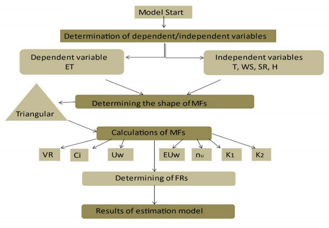
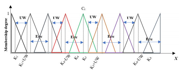
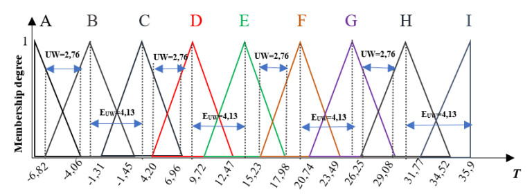
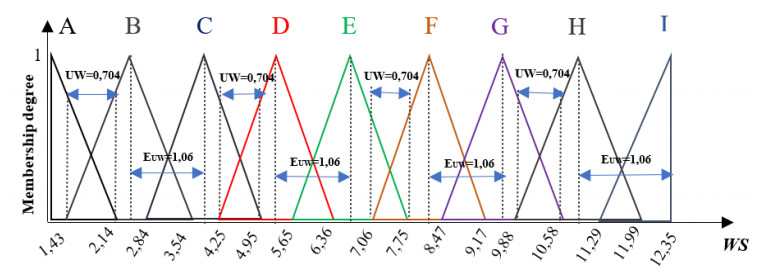
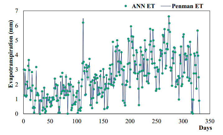
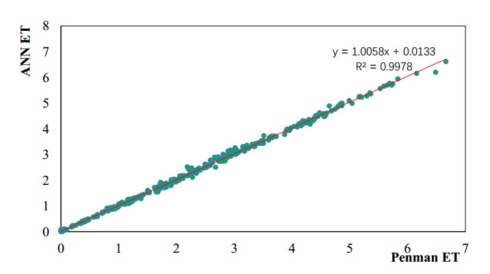
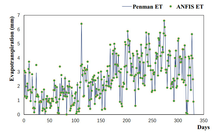
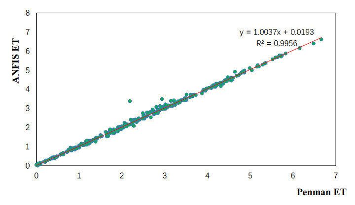
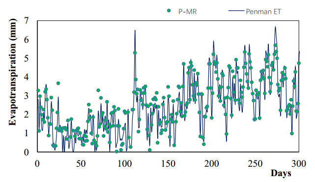
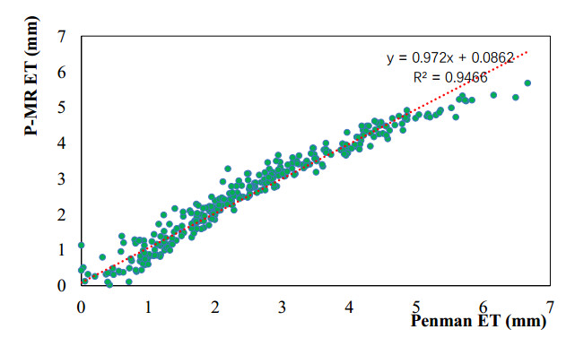
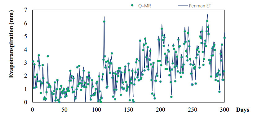
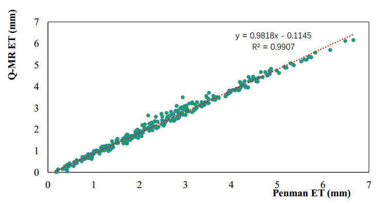
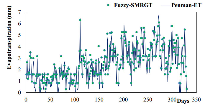
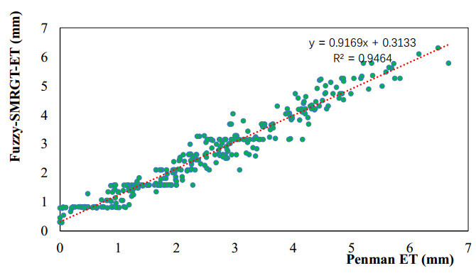
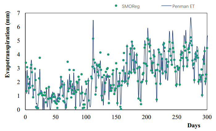
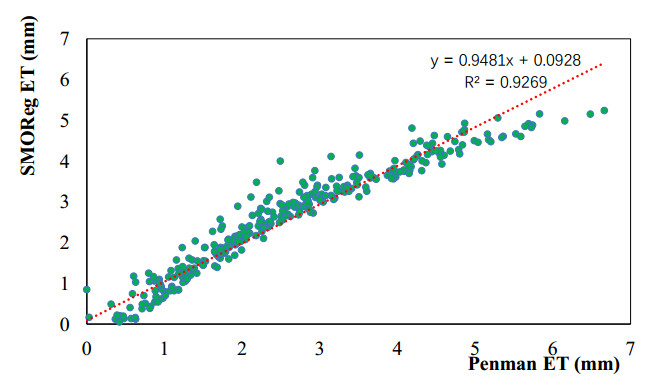
Evapotranspiration is an important parameter to be considered in hydrology. In the design of water structures, accurate estimation of the amount of evapotranspiration allows for safer designs. Thus, maximum efficiency can be obtained from the structure. In order to accurately estimate evapotranspiration, the parameters affecting evapotranspiration should be well known. There are many factors that affect evapotranspiration. Some of these can be listed as temperature, humidity in the atmosphere, wind speed, pressure and water depth. In this study, models were created for the estimation of the daily evapotranspiration amount by using the simple membership functions and fuzzy rules generation technique (fuzzy-SMRGT), multivariate regression (MR), artificial neural networks (ANNs), adaptive neuro-fuzzy inference system (ANFIS) and support vector regression (SMOReg) methods. Model results were compared with each other and traditional regression calculations. The ET amount was calculated empirically using the Penman-Monteith (PM) method which was taken as a reference equation. In the created models, daily air temperature (T), wind speed (WS), solar radiation (SR), relative humidity (H) and evapotranspiration (ET) data were obtained from the station near Lake Lewisville (Texas, USA). The coefficient of determination (R2), root mean square error (RMSE) and average percentage error (APE) were used to compare the model results. According to the performance criteria, the best model was obtained by Q-MR (quadratic-MR), ANFIS and ANN methods. The R2, RMSE, APE values of the best models were 0,991, 0,213, 18,881% for Q-MR; 0,996; 0,103; 4,340% for ANFIS and 0,998; 0,075; 3,361% for ANN, respectively. The Q-MR, ANFIS and ANN models had slightly better performance than the MLR, P-MR and SMOReg models.
Citation: Hasan Güzel, Fatih Üneş, Merve Erginer, Yunus Ziya Kaya, Bestami Taşar, İbrahim Erginer, Mustafa Demirci. A comparative study on daily evapotranspiration estimation by using various artificial intelligence techniques and traditional regression calculations[J]. Mathematical Biosciences and Engineering, 2023, 20(6): 11328-11352. doi: 10.3934/mbe.2023502
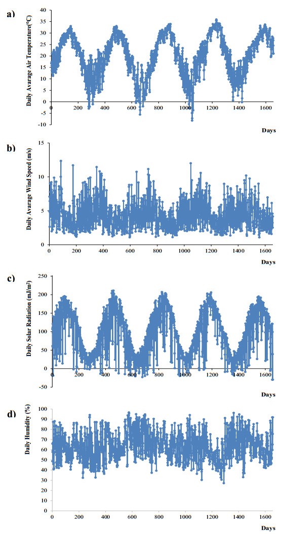
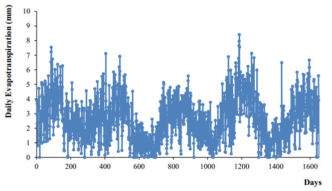
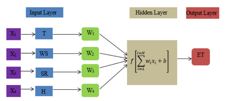
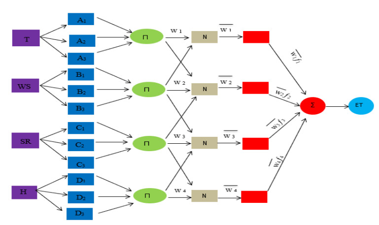
Evapotranspiration is an important parameter to be considered in hydrology. In the design of water structures, accurate estimation of the amount of evapotranspiration allows for safer designs. Thus, maximum efficiency can be obtained from the structure. In order to accurately estimate evapotranspiration, the parameters affecting evapotranspiration should be well known. There are many factors that affect evapotranspiration. Some of these can be listed as temperature, humidity in the atmosphere, wind speed, pressure and water depth. In this study, models were created for the estimation of the daily evapotranspiration amount by using the simple membership functions and fuzzy rules generation technique (fuzzy-SMRGT), multivariate regression (MR), artificial neural networks (ANNs), adaptive neuro-fuzzy inference system (ANFIS) and support vector regression (SMOReg) methods. Model results were compared with each other and traditional regression calculations. The ET amount was calculated empirically using the Penman-Monteith (PM) method which was taken as a reference equation. In the created models, daily air temperature (T), wind speed (WS), solar radiation (SR), relative humidity (H) and evapotranspiration (ET) data were obtained from the station near Lake Lewisville (Texas, USA). The coefficient of determination (R2), root mean square error (RMSE) and average percentage error (APE) were used to compare the model results. According to the performance criteria, the best model was obtained by Q-MR (quadratic-MR), ANFIS and ANN methods. The R2, RMSE, APE values of the best models were 0,991, 0,213, 18,881% for Q-MR; 0,996; 0,103; 4,340% for ANFIS and 0,998; 0,075; 3,361% for ANN, respectively. The Q-MR, ANFIS and ANN models had slightly better performance than the MLR, P-MR and SMOReg models.

| [1] | C. İnal, P. Fakioğlu, S. Bülbül, Determination of sediment volumes in dams with hydrographic surveys, Selcuk University J. Eng. Sci. Technol., 3 (2015), 1–12. https://dergipark.org.tr/en/pub/sujest/issue/23197/247765 (accessed March, 2023) |
| [2] |
B. Taşar, F. Üneş, M. Demi̇rci̇, Y. Z. Kaya, Forecasting of daily evaporation amounts using artificial neural networks technique, Dicle University J. Eng., 9 (2018), 543–551. https://doi.org/10.1002/CLEN.200900238 doi: 10.1002/CLEN.200900238

|
| [3] |
Y. Z. Kaya, M. Zelenakova, F. Üneş, M. Demirci, H. Hlavata, P. Mesaros, Estimation of daily evapotranspiration in Košice City (Slovakia) using several soft computing techniques, Theor. Appl. Climatol., 144 (2021), 287–298. https://doi.org/10.1007/S00704-021-03525-Z doi: 10.1007/S00704-021-03525-Z
|
| [4] |
F. Üneş, Y. Z. Kaya, M. Mamak, Daily reference evapotranspiration prediction based on climatic conditions applying different data mining techniques and empirical equations, Theor. Appl. Climatol., 141 (2020), 763–773. https://doi.org/10.1007/S00704-020-03225-0/TABLES/4 doi: 10.1007/S00704-020-03225-0/TABLES/4
|
| [5] |
M. Demirci, F. Üneş, S. Körlü, Modeling of groundwater level using artificial intelligence techniques: A case study of Reyhanli region in Turkey, Appl. Ecol. Environ. Res., 17 (2019), 2651–2663. https://doi.org/10.15666/AEER/1702_26512663 doi: 10.15666/AEER/1702_26512663
|
| [6] | F. Üneş, B. Taşar, M. Demirci, M. Zelenakova, Y. Z. Kaya, H. Varçin, Daily suspended sediment prediction using seasonal time series and artificial intelligence techniques, Rocznik Ochrona Środowiska, 23 (2021). https://doi.org/10.54740/ros.2021.008 |
| [7] |
H. S. Choi, J. H. Kim, E. H. Lee, S. K. Yoon, Development of a revised multi-layer perceptron model for dam inflow prediction, Water, 14 (2022), 1878. https://doi.org/10.3390/W14121878 doi: 10.3390/W14121878
|
| [8] |
H. Leyla, S. Nadia, R. Bouchrit, Modeling and predictive analyses related to piezometric level in an earth dam using a back propagation neural network in comparison on non-linear regression, Model. Earth Syst. Environ., 9 (2022), 1169–1180. https://doi.org/10.1007/S40808-022-01558-5 doi: 10.1007/S40808-022-01558-5
|
| [9] |
Y. Ouma, D. Moalafhi, G. Anderson, B. Nkwae, P. Odirile, B. P. Parida, et al., Dam water level prediction using vector autoregression, random forest regression and MLP-ANN models based on Land-use and climate factors, Sustainability, 14 (2022), 14934. https://doi.org/10.3390/su142214934 doi: 10.3390/su142214934
|
| [10] |
M. Guermoui, F. Melgani, K. Gairaa, M. L. Mekhalfi, A comprehensive review of hybrid models for solar radiation forecasting, J. Clean. Prod., 258 (2020), 120357. https://doi.org/10.1016/J.JCLEPRO.2020.120357 doi: 10.1016/J.JCLEPRO.2020.120357
|
| [11] |
M. Guermoui, S. Benkaciali, K. Gairaa, K. Bouchouicha, T. Boulmaiz, J. W. Boland, A novel ensemble learning approach for hourly global solar radiation forecasting, Neural Comput. Appl., 34 (2022), 2983–3005. https://doi.org/10.1007/S00521-021-06421-9 doi: 10.1007/S00521-021-06421-9
|
| [12] |
M. Guermoui, K. Gairaa, K. Ferkous, D. S. O. Santos, T. Arrif, A. Belaid, Potential assessment of the TVF-EMD algorithm in forecasting hourly global solar radiation: Review and case studies, J. Clean. Prod. , 385 (2023), 135680. https://doi.org/10.1016/j.jclepro.2022.135680 doi: 10.1016/j.jclepro.2022.135680
|
| [13] |
I. Karatas, A. Budak, Prediction of labor activity recognition in construction with machine learning algorithms, Icontech Int. J. , 5 (2021), 38–47. https://doi.org/10.46291/ICONTECHvol5iss3pp38-47 doi: 10.46291/ICONTECHvol5iss3pp38-47
|
| [14] |
C. Kayadelen, G. Altay, S. Önal, Y. Önal, Sequential minimal optimization for local scour around bridge piers, Mar. Georesour. Geotec., 40 (2021), 462–472. https://doi.org/10.1080/1064119X.2021.1907635 doi: 10.1080/1064119X.2021.1907635
|
| [15] |
C. Kayadelen, G. Altay, Y. Önal, Numerical simulation and novel methodology on resilient modulus for traffic loading on road embankment, Int. J. Pavem. Eng., 23 (2021), 3212–3221. https://doi.org/10.1080/10298436.2021.1886296 doi: 10.1080/10298436.2021.1886296
|
| [16] |
M. Demirci, A. Baltaci, Prediction of suspended sediment in river using fuzzy logic and multilinear regression approaches, Neural Comput. Appl., 23 (2013), 145–151. https://doi.org/10.1007/S00521-012-1280-Z doi: 10.1007/S00521-012-1280-Z
|
| [17] |
M. Achite, M. Jehanzaib, M. T. Sattari, A. K. Toubal, N. Elshaboury, A. Wałęga, et al., Modern techniques to modeling reference evapotranspiration in a semiarid area based on ANN and GEP models, Water, 14 (2022), 1210. https://doi.org/10.3390/W14081210 doi: 10.3390/W14081210
|
| [18] | F. Üneş, S. Doğan, B. Taşar, Y. Z. Kaya, M. Demirci, The evaluation and comparison of daily reference evapotranspiration with ANN and empirical methods, Nat. Eng. Sci. , 3 (2018), 54–64. |
| [19] |
H. Tao, L. Diop, A. Bodian, K. Djaman, P. M. Ndiaye, Z. M. Yaseen, Reference evapotranspiration prediction using hybridized fuzzy model with firefly algorithm: Regional case study in Burkina Faso, Agr. Water Manag., 208 (2018), 140–151. https://doi.org/10.1016/J.AGWAT.2018.06.018 doi: 10.1016/J.AGWAT.2018.06.018
|
| [20] |
G. Huang, L. Wu, X. Ma, W. Zhang, J. Fan, X. Yu, et al., Evaluation of CatBoost method for prediction of reference evapotranspiration in humid regions, J. Hydrol., 574 (2019), 1029–1041. https://doi.org/10.1016/J.JHYDROL.2019.04.085 doi: 10.1016/J.JHYDROL.2019.04.085
|
| [21] | M. Kadkhodazadeh, M. V. Anaraki, A. Morshed-Bozorgdel, S. Farzin, A new methodology for reference evapotranspiration prediction and uncertainty analysis under climate change conditions based on machine learning, multi criteria decision making and Monte Carlo methods, Sustainability, 14 (2022), 2601. https://doi.org/10.3390/SU14052601 |
| [22] |
M. Chia, Y. Huang, C. Koo, J. Ng, A. Ahmed, A. El-Shafie, Long-term forecasting of monthly mean reference evapotranspiration using deep neural network: A comparison of training strategies and approaches, Appl. Soft Comput. , 126 (2022), 109221. https://doi.org/10.1016/j.asoc.2022.109221 doi: 10.1016/j.asoc.2022.109221
|
| [23] |
Y. Z. Kaya, M. Mamak, F. Üneş, Evapotranspiration prediction using M5T data mining method, Ijaers J., 3 (2016), 2456–1908. https://doi.org/10.22161/ijaers/3.12.40 doi: 10.22161/ijaers/3.12.40
|
| [24] | D. Yildirim, B. Cemek, E. Küçüktopcu, Estimation of daily evaporation using fuzzy artificial neural network (ANFIS) and multilayer artificial neural network system (ANN), Toprak Su J., (2019), 24–31, (in Turkish). https://doi.org/10.21657/TOPRAKSU.654778 |
| [25] |
A. Ozel, M. Buyukyildiz, Usability of artificial intelligence methods for estimation of monthly evaporation, Omer Halisdemir University J. Eng. Sci. , 8 (2019), 244–254. https://doi.org/10.28948/NGUMUH.516891 doi: 10.28948/NGUMUH.516891
|
| [26] |
Z. F. Toprak, Flow discharge modeling in open canals using a new fuzzy modeling technique (SMRGT), CLEAN–Soil Air Water, 37 (2009), 742–752. https://doi.org/10.1002/CLEN.200900146 doi: 10.1002/CLEN.200900146
|
| [27] | E. Altaş, M. C. Aydın, Z. F. Toprak, Modeling Water surface profile in open channel flows using fuzzy SMRGT method, Dicle University J. Eng., 9 (2018), 975–981. |
| [28] | USGS. gov | Science for a changing world, (n.d.). https://www.usgs.gov/. |
| [29] |
H. L. Penman, Natural evaporation from open water, hare soil and grass, Proc. R Soc. Lond. A Math. Phys. Sci., 193 (1948), 120–145. https://doi.org/10.1098/RSPA.1948.0037 doi: 10.1098/RSPA.1948.0037
|
| [30] | M. Jensen, R. Burman, R. Allen, Evapotranspiration and irrigation water requirements, ASCE, New York, (1990). https://cedb.asce.org/CEDBsearch/record.jsp?dockey = 0067841 |
| [31] |
F. Cansiz, F. Üneş, I. Erginer, B. Taşar, Modeling of highways energy consumption with artificial intelligence and regression methods, Int. J. Environ. Sci. Technol. , 19 (2022), 9741–9756. https://doi.org/10.1007/S13762-021-03813-1 doi: 10.1007/S13762-021-03813-1
|
| [32] |
Ö. F. Cansiz, İ. Ergi̇ner, E. Doğru, Estimation number of traffic accidents and number of injured by artificial neural networks and regression methods, Osmaniye Korkut Ata University J. Inst. Sci. Technol. , 3 (2020), 29–35. https://doi.org/10.47495/OKUFBED.844250 doi: 10.47495/OKUFBED.844250
|
| [33] |
C. Riviere, P. Lauret, J. F. M. Ramsamy, Y. Page, A Bayesian Neural Network approach to estimating the Energy Equivalent Speed, Accid Anal. Prev. , 38 (2006), 248–259. https://doi.org/10.1016/J.AAP.2005.08.008 doi: 10.1016/J.AAP.2005.08.008
|
| [34] | N. Walia, H. Singh, A. Sharma, ANFIS: Adaptive neuro-fuzzy inference system-a survey, Int. J. Comput. Appl. , 123 (2015), 32–38. |
| [35] |
F. Üneş, M. Demirci, M. Zelenakova, M. Çalişici, B. Taşar, F. Vranay, et al., river flow estimation using artificial intelligence and fuzzy techniques, Water, 12 (2020), 2427. https://doi.org/10.3390/W12092427 doi: 10.3390/W12092427
|
| [36] | J. S. R. Jang, Fuzzy modeling using generalized neural networks and Kalman filter algorithm, In AAAI-91 Proceedings, (1991), 762–767. |
| [37] | J. S. R. Jang, ANFIS: Adaptive-network-based fuzzy inference system, IEEE Transact. Syst. Man. Cybernet. , 23 (1993), 665–685. |
| [38] | Z. F. Toprak, A. Toprak, Z. Aykac, Practical applications of Fuzzy SMRGT method, Dicle University J. Eng. , 8 (2017), 123–132. |
| [39] |
S. K. Shevade, S. S. Keerthi, C. Bhattacharyya, K. R. K. Murthy, Improvements to the SMO algorithm for SVM regression, IEEE Trans. Neural Netw. , 11 (2000), 1188–1193. https://doi.org/10.1109/72.870050 doi: 10.1109/72.870050
|
| [40] | A. J. Smola, B. Schoelkopf, A tutorial on support vector regression, 1998. |

Figures(29) / Tables(1)

Hasan Güzel, Fatih Üneş, Merve Erginer, Yunus Ziya Kaya, Bestami Taşar, İbrahim Erginer, Mustafa Demirci. A comparative study on daily evapotranspiration estimation by using various artificial intelligence techniques and traditional regression calculations[J]. Mathematical Biosciences and Engineering, 2023, 20(6): 11328-11352. doi: 10.3934/mbe.2023502


 DownLoad: