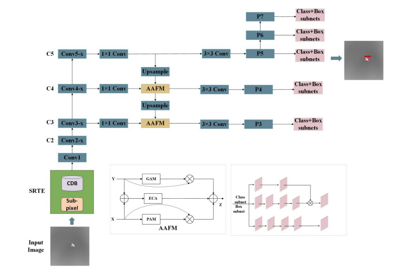
To solve the problems of texture lacking and resolution coarseness in the detection of dim and small drone targets in infrared images, we propose a novel RetinaNet with an asymmetric attention fusion mechanism for dim and small drone detection. First, we propose a super-resolution texture-enhancement network as an effective solution for the lack of texture-related information on small infrared targets. The network generates super-resolution images and enhances the texture features of the targets. Second, considering the inadequacy of feature pyramids in the feature fusion stage, we use an asymmetric attention fusion mechanism to constitute an asymmetric attention fusion pyramid network for cross-layer feature fusion in a bidirectional manner; it achieves high-quality semantic and location detail information interaction between scale features. Third, a global average pooling layer is employed to capture global spatial-sensitive information, thus effectively identifying features and achieving classification. Experiments were conducted by using a publicly available infrared image dim-small drone target detection dataset; the results show that the proposed method achieves an AP of 95.43% and a recall of 80.6%, which is a significant improvement over the current mainstream target detection algorithms.
Citation: Zhijing Xu, Jingjing Su, Kan Huang. A-RetinaNet: A novel RetinaNet with an asymmetric attention fusion mechanism for dim and small drone detection in infrared images[J]. Mathematical Biosciences and Engineering, 2023, 20(4): 6630-6651. doi: 10.3934/mbe.2023285
To solve the problems of texture lacking and resolution coarseness in the detection of dim and small drone targets in infrared images, we propose a novel RetinaNet with an asymmetric attention fusion mechanism for dim and small drone detection. First, we propose a super-resolution texture-enhancement network as an effective solution for the lack of texture-related information on small infrared targets. The network generates super-resolution images and enhances the texture features of the targets. Second, considering the inadequacy of feature pyramids in the feature fusion stage, we use an asymmetric attention fusion mechanism to constitute an asymmetric attention fusion pyramid network for cross-layer feature fusion in a bidirectional manner; it achieves high-quality semantic and location detail information interaction between scale features. Third, a global average pooling layer is employed to capture global spatial-sensitive information, thus effectively identifying features and achieving classification. Experiments were conducted by using a publicly available infrared image dim-small drone target detection dataset; the results show that the proposed method achieves an AP of 95.43% and a recall of 80.6%, which is a significant improvement over the current mainstream target detection algorithms.

| [1] |
X. Shao, H. Fan, G. Lu, J. Xu, An improved infrared dim and small target detection algorithm based on the contrast mechanism of human visual system, Infrared Phys. Technol., 55 (2012), 403–408. https://doi.org/10.1016/j.infrared.2012.06.001 doi: 10.1016/j.infrared.2012.06.001

|
| [2] |
M. Fan, S. Tian, K. Liu, J. Zhao, Y. Li, Infrared small target detection based on region proposal and CNN classifier, Signal, Image Video Process., 15 (2021), 1927–1936. https://doi.org/10.1007/s11760-021-01936-z doi: 10.1007/s11760-021-01936-z
|
| [3] |
Y. Zhang, L. Zheng, Y. Zhang, Small infrared target detection via a Mexican-Hat distribution, Appl. Sci., 9 (2019). https://doi.org/10.3390/app9245570 doi: 10.3390/app9245570
|
| [4] |
X. Cao, C. Rong, X. Bai, Infrared small target detection based on derivative dissimilarity measure, IEEE J. Sel. Top. Appl. Earth Obs. Remote Sens., 12 (2019), 3101–3116. https://doi.org/10.1109/JSTARS.2019.2920327 doi: 10.1109/JSTARS.2019.2920327
|
| [5] |
C. Chen, H. Li, Y. Wei, T. Xia, Y. Tang, A local contrast method for small infrared target detection, IEEE Trans. Geosci. Remote Sens., 52 (2014), 574–581. https://doi.org/10.1109/TGRS.2013.2242477 doi: 10.1109/TGRS.2013.2242477
|
| [6] |
J. Han, Y. Ma, B. Zhou, F. Fan, K. Liang, Y. Fang, A robust infrared small target detection algorithm based on human visual system, IEEE Geosci. Remote Sens. Lett., 11 (2014), 2168–2172. https://doi.org/10.1109/LGRS.2014.2323236 doi: 10.1109/LGRS.2014.2323236
|
| [7] |
Y. Qin, B. Li, Effective infrared small target detection utilizing a novel local contrast method, IEEE Geosci. Remote Sens. Lett., 13 (2016), 1890–1894. https://doi.org/10.1109/LGRS.2016.2616416 doi: 10.1109/LGRS.2016.2616416
|
| [8] |
L. Wu, Y. Ma, F. Fan, M. Wu, J. Huang, A double-neighborhood gradient method for infrared small target detection, IEEE Geosci. Remote Sens. Lett., 18 (2021), 1476–1480. https://doi.org/10.1109/LGRS.2020.3003267 doi: 10.1109/LGRS.2020.3003267
|
| [9] |
Y. Lu, L. Dong, T. Zhang, W. Xu, A robust detection algorithm for infrared maritime small and dim targets, Sensors, 20 (2020). https://doi.org/10.3390/s20041237 doi: 10.3390/s20041237
|
| [10] |
X. Wang, Z. Peng, D. Kong, Y. He, Infrared dim and small target detection based on stable multisubspace learning in heterogeneous scene, IEEE Trans. Geosci. Remote Sens., 55 (2017), 5481–5493. https://doi.org/10.1109/TGRS.2017.2709250 doi: 10.1109/TGRS.2017.2709250
|
| [11] |
L. Dong, B. Wang, M. Zhao, W. Xu, Robust infrared maritime target detection based on visual attention and spatiotemporal filtering, IEEE Trans. Geosci. Remote Sens., 55 (2017), 3037–3050. https://doi.org/10.1109/TGRS.2017.2660879 doi: 10.1109/TGRS.2017.2660879
|
| [12] |
L. Ding, X. Xu, Y. Cao, G. Zhai, F. Yang, L. Qian, Detection and tracking of infrared small target by jointly using SSD and pipeline filter, Digital Signal Process., 110 (2021). https://doi.org/10.1016/j.dsp.2020.102949 doi: 10.1016/j.dsp.2020.102949
|
| [13] |
Q. Guo, Z. Li, W. Song, W. Fu, Parallel computing based dynamic programming algorithm of track-before-detect, Symmetry, 11 (2019). https://doi.org/10.3390/sym11010029 doi: 10.3390/sym11010029
|
| [14] |
Q. Hu, J. Yang, P. Qin, S. Fong, Towards a context-free machine universal grammar (CF-MUG) in natural language processing, IEEE Access, 8 (2020). https://doi.org/10.1109/ACCESS.2020.3022674 doi: 10.1109/ACCESS.2020.3022674
|
| [15] |
A. Ilioudi, A. Dabiri, B. J. Wolf, B. De Schutter, Deep learning for object detection and segmentation in videos: toward an integration with domain knowledge, IEEE Access, 10 (2022), 34562–34576. https://doi.org/10.1109/ACCESS.2022.3162827 doi: 10.1109/ACCESS.2022.3162827
|
| [16] | R. Girshick, J. Donahue, T. Darrell, J. Malik, Rich feature hierarchies for accurate object detection and semantic segmentation, in 2014 IEEE Conference on Computer Vision and Pattern Recognition, (2014), 580–587. https://doi.org/10.1109/CVPR.2014.81 |
| [17] | R. Girshick, Fast R-CNN, in 2015 IEEE International Conference on Computer Vision (ICCV), (2015), 7–13. https://doi.org/10.1109/ICCV.2015.169 |
| [18] |
S. Ren, K. He, R. Girshick, J. Sun, Faster R-CNN: Towards real-time object detection with region proposal networks, IEEE Trans. Pattern Anal. Mach. Intell., 39 (2017), 1137–1149. https://doi.org/10.1109/TPAMI.2016.2577031 doi: 10.1109/TPAMI.2016.2577031
|
| [19] | W. Liu, A. Dragomir, E. Dumitru, S. Christian, R. Scott, C. Fu, et al., SSD: Single shot multibox detector, in Lecture Notes in Computer Science, (2016), 21–37. https://doi.org/10.1007/978-3-319-46448-0_2 |
| [20] | J. Redmon, A. Farhadi, YOLOV3: An incremental improvement, arXiv preprints, (2018), arXiv: 1804.02767. https://doi.org/10.48550/arXiv.1804.02767 |
| [21] | T. Y. Lin, P. Goyal, R. Girshick, K. He, P. Dollár, Focal loss for dense object detection, in 2017 IEEE International Conference on Computer Vision (ICCV), (2017), 2999–3007. https://doi.org/10.1109/ICCV.2017.324 |
| [22] |
M. Ju, J. Luo, P. Zhang, M. He, H. Luo, A simple and efficient network for small target detection, IEEE Access, 7 (2019), 85771–85781. https://doi.org/10.1109/ACCESS.2019.2924960 doi: 10.1109/ACCESS.2019.2924960
|
| [23] |
H. Liang, J. Yang, M. Shao, FE-RetinaNet: small target detection with parallel multi-scale feature enhancement, Symmetry, 13 (2021). https://doi.org/10.3390/sym13060950 doi: 10.3390/sym13060950
|
| [24] |
Q. Hou, Z. Wang, F. Tan, Y. Zhao, H. Zheng, W. Zhang, RISTDnet: Robust infrared small target detection network, IEEE Geosci. Remote Sens. Lett., 19 (2021), 1–5. https://doi.org/10.1109/LGRS.2021.3050828 doi: 10.1109/LGRS.2021.3050828
|
| [25] |
Y. Li, S. Li, H. Du, L. Chen, D. Zhang, Y. Li. YOLO-ACN: Focusing on small target and occluded object detection, IEEE Access, 8 (2020), 227288–227303. https://doi.org/10.1109/ACCESS.2020.3046515 doi: 10.1109/ACCESS.2020.3046515
|
| [26] |
Z. Song, Y. Zhang, Y. Liu, K. Yang, M. Sun, MSFYOLO: Feature fusion-based detection for small objects, IEEE Lat. Am. Trans., 20 (2022), 823–830. https://doi.org/10.1109/TLA.2022.9693567 doi: 10.1109/TLA.2022.9693567
|
| [27] |
K. Wang, S. Li, S. Niu, K. Zhang, Detection of infrared small targets using feature fusion convolutional network, IEEE Access, 7 (2019), 146081–146092. https://doi.org/10.1109/ACCESS.2019.2944661 doi: 10.1109/ACCESS.2019.2944661
|
| [28] |
M. Ju, J. Luo, G. Liu, H. Luo, ISTDet: An efficient end-to-end neural network for infrared small target detection, Infrared Phys. Technol., 114 (2021). https://doi.org/10.1016/j.infrared.2021.103659 doi: 10.1016/j.infrared.2021.103659
|
| [29] |
S. Yao, Q. Zhu, T. Zhang, W. Cui, P. Yan, Infrared image small-target detection based on improved FCOS and spatio-temporal features, Electronics, 11 (2022). https://doi.org/10.3390/electronics11060933 doi: 10.3390/electronics11060933
|
| [30] |
X. Tong, B. Sun, J. Wei, Z. Zuo, S. Su, EAAU-Net: Enhanced asymmetric attention U-Net for infrared small target detection, Remote Sens., 13 (2021). https://doi.org/10.3390/rs13163200 doi: 10.3390/rs13163200
|
| [31] |
Q. Xu, H. Huang, C. Zhou, X. Zhang, Research on real-time infrared image fault detection of substation high-voltage lead connectors based on improved YOLOv3 network, Electronics, 10 (2021). https://doi.org/10.3390/electronics10050544 doi: 10.3390/electronics10050544
|
| [32] |
C. Deng, M. Wang, L. Liu, Y. Liu, Y. Jiang, Extended feature pyramid network for small object detection, IEEE Trans. Multimedia, 24 (2021), 1968–1979. https://doi.org/10.1109/TMM.2021.3074273 doi: 10.1109/TMM.2021.3074273
|
| [33] | G. Huang, Z. Liu, L. Van Der Maaten, K. Q. Weinberger, Densely connected convolutional networks, in 2017 IEEE Conference on Computer Vision and Pattern Recognition (CVPR), (2017), 2261–2269. https://doi.org/10.1109/CVPR.2017.243 |
| [34] | Y. Dai, Y. Wu, F. Zhou, K. Barnard, Asymmetric contextual modulation for infrared small target detection, in 2021 IEEE Winter Conference on Applications of Computer Vision (WACV), (2021), 949–958. https://doi.org/10.1109/WACV48630.2021.00099 |
| [35] | Q. Wang, B. Wu, P. Zhu, P. Li, W. Zuo, Q. Hu, ECA-Net: Efficient channel attention for deep convolutional neural networks, in 2020 IEEE/CVF Conference on Computer Vision and Pattern Recognition (CVPR), (2020), 11531–11539. https://doi.org/10.1109/CVPR42600.2020.01155 |
| [36] | M. Pastorino, G. Moser, S. B. Serpico, J. Zerubia, Fully convolutional and feedforward networks for the semantic segmentation of remotely sensed images, in 2022 IEEE International Conference on Image Processing (ICIP), (2022), 1876–1880. https://doi.org/10.1109/ICIP46576.2022.9897336 |
| [37] | M. Lin, Q. Chen, S. Yan, Network in network, arXiv preprints, (2013), arXiv: 1312.4400. https://doi.org/10.48550/arXiv.1312.4400 |
| [38] | B. Hui, Z. Song, H. Fan, P. Zhong, W. Hu, X. Zhang, et al., A dataset for infrared image dim-small aircraft target detection and tracking under ground/air background, Science Data Bank, (2019). https://doi.org/10.11922/sciencedb |
| [39] | X. Zhou, D. Wang, P. Krähenbähl, Objects as points, arXiv preprint, (2019), arXiv: 1904.07850. http://arXiv.org/abs/1904.07850 |


Figures(14) / Tables(4)

Zhijing Xu, Jingjing Su, Kan Huang. A-RetinaNet: A novel RetinaNet with an asymmetric attention fusion mechanism for dim and small drone detection in infrared images[J]. Mathematical Biosciences and Engineering, 2023, 20(4): 6630-6651. doi: 10.3934/mbe.2023285


 DownLoad: