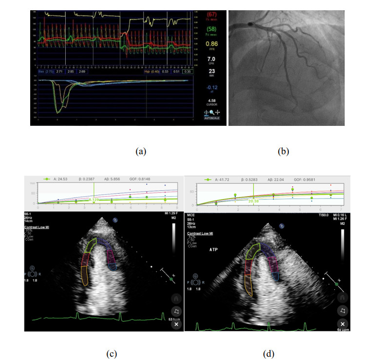
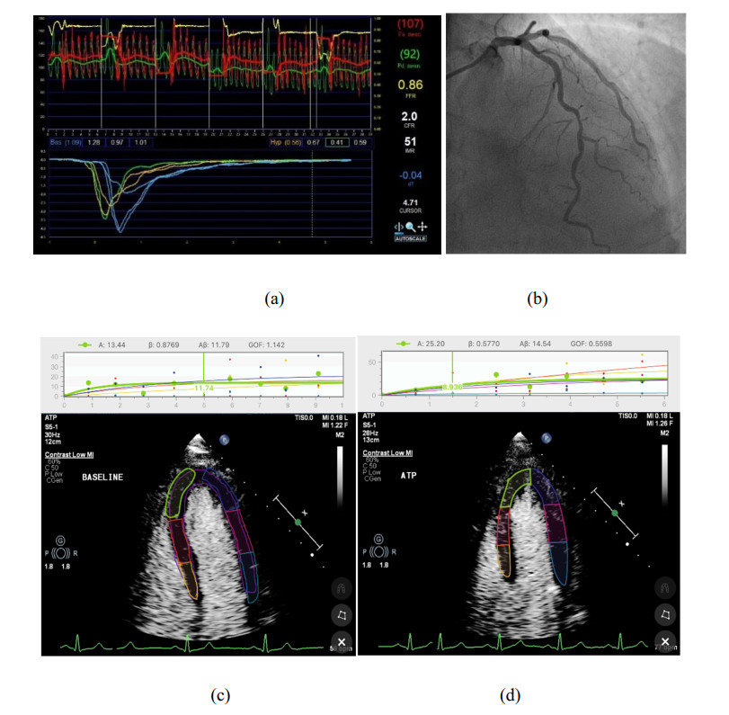
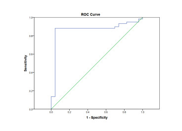
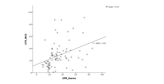
Coronary microvascular dysfunction (CMD) is one of the basic mechanisms of myocardial ischemia. Myocardial contrast echocardiography (MCE) is a bedside technique that utilises microbubbles which remain entirely within the intravascular space and denotes the status of microvascular perfusion within that region. Some pilot studies suggested that MCE may be used to diagnose CMD, but without further validation. This study is aimed to investigate the diagnostic performance of MCE for the evaluation of CMD. MCE was performed at rest and during adenosine triphosphate stress. ECG triggered real-time frames were acquired in the apical 4-chamber, 3-chamber, 2-chamber, and long-axis imaging planes. These images were imported into Narnar for further processing. Eighty-two participants with suspicion of coronary disease and absence of significant epicardial lesions were prospectively investigated. Thermodilution was used as the gold standard to diagnose CMD. CMD was present in 23 (28%) patients. Myocardial blood flow reserve (MBF) was assessed using MCE. CMD was defined as MBF reserve < 2. The MCE method had a high sensitivity (88.1%) and specificity (95.7%) in the diagnosis of CMD. There was strong agreement with thermodilution (Kappa coefficient was 0.727; 95% CI: 0.57–0.88, p < 0.001). However, the correlation coefficient (r = 0.376; p < 0.001) was not high.
Citation: Jucheng Zhang, Minwen Ma, Huajun Li, Zhaoxia Pu, Haipeng Liu, Tianhai Huang, Huan Cheng, Yinglan Gong, Yonghua Chu, Zhikang Wang, Jun Jiang, Ling Xia. Early diagnosis of coronary microvascular dysfunction by myocardial contrast stress echocardiography[J]. Mathematical Biosciences and Engineering, 2023, 20(5): 7845-7858. doi: 10.3934/mbe.2023339
Coronary microvascular dysfunction (CMD) is one of the basic mechanisms of myocardial ischemia. Myocardial contrast echocardiography (MCE) is a bedside technique that utilises microbubbles which remain entirely within the intravascular space and denotes the status of microvascular perfusion within that region. Some pilot studies suggested that MCE may be used to diagnose CMD, but without further validation. This study is aimed to investigate the diagnostic performance of MCE for the evaluation of CMD. MCE was performed at rest and during adenosine triphosphate stress. ECG triggered real-time frames were acquired in the apical 4-chamber, 3-chamber, 2-chamber, and long-axis imaging planes. These images were imported into Narnar for further processing. Eighty-two participants with suspicion of coronary disease and absence of significant epicardial lesions were prospectively investigated. Thermodilution was used as the gold standard to diagnose CMD. CMD was present in 23 (28%) patients. Myocardial blood flow reserve (MBF) was assessed using MCE. CMD was defined as MBF reserve < 2. The MCE method had a high sensitivity (88.1%) and specificity (95.7%) in the diagnosis of CMD. There was strong agreement with thermodilution (Kappa coefficient was 0.727; 95% CI: 0.57–0.88, p < 0.001). However, the correlation coefficient (r = 0.376; p < 0.001) was not high.

| [1] |
P. G. Camici, F. Crea, Coronary microvascular dysfunction, N. Engl. J. Med., 356 (2007), 830–840. https://doi.org/10.1056/NEJMra061889 doi: 10.1056/NEJMra061889

|
| [2] |
G. Montalescot, U. Sechtem, S. Achenbach, F. Andreotti, C. Arden, A. Budaj, et al., 2013 ESC guidelines on the management of stable coronary artery disease: the Task Force on the management of stable coronary artery disease of the European Society of Cardiology, Eur. Heart J., 34 (2013), 2949–3003. https://doi.org/10.1093/eurheartj/eht296 doi: 10.1093/eurheartj/eht296
|
| [3] |
T. J. Ford, E. Yii, N. Sidik, R. Good, P. Rocchiccioli, M. McEntegart, et al., Ischemia and no obstructive coronary artery disease: prevalence and correlates of coronary vasomotion disorders, Circ. Cardiovasc. Interventions, 12 (2019), e008126. https://doi.org/10.1161/CIRCINTERVENTIONS.119.008126 doi: 10.1161/CIRCINTERVENTIONS.119.008126
|
| [4] |
C. L. Schumann, R. C. Mathew, J. L. Dean, Y. Yang, P. C. Balfour, P. W. Shaw, et al., Functional and economic impact of INOCA and influence of coronary microvascular dysfunction, JACC Cardiovasc. Imaging, 14 (2021), 1369–1379. https://doi.org/10.1016/j.jcmg.2021.01.041 doi: 10.1016/j.jcmg.2021.01.041
|
| [5] |
J. C. Kaski, F. Crea, B. J. Gersh, P. G. Camici, Reappraisal of ischemic heart disease, Circulation, 138 (2018), 1463–1480. https://doi.org/10.1161/CIRCULATIONAHA.118.031373 doi: 10.1161/CIRCULATIONAHA.118.031373
|
| [6] |
H. Shimokawa, A. Suda, J. Takahashi, C. Berry, P. G. Camici, F. Crea, et al., Clinical characteristics and prognosis of patients with microvascular angina: an international and prospective cohort study by the Coronary Vasomotor Disorders International Study (COVADIS) Group, Eur. Heart J., 42, (2021), 4592–4600. https://doi.org/10.1093/eurheartj/ehab282 doi: 10.1093/eurheartj/ehab282
|
| [7] |
L. J. Shaw, C. N. Merz, C. J. Pepine, S. E. Reis, V. Bittner, K. E. Kip, et al., The economic burden of angina in women with suspected ischemic heart disease, Circulation, 114 (2006), 894–904. https://doi.org/10.1161/CIRCULATIONAHA.105.609990 doi: 10.1161/CIRCULATIONAHA.105.609990
|
| [8] |
G. A. Lanza, D. Morrone, C. Pizzi, I. Tritto, L. Bergamaschi, A. De Vita, et al., Diagnostic approach for coronary microvascular dysfunction in patients with chest pain and no obstructive coronary artery disease, Trends Cardiovasc. Med., 32 (2022), 448–453. https://doi.org/10.1016/j.tcm.2021.08.005 doi: 10.1016/j.tcm.2021.08.005
|
| [9] |
P. Ong, B. Safdar, A. Seitz, A. Hubert, J. F. Beltrame, E. Prescott, Diagnosis of coronary microvascular dysfunction in the clinic, Cardiovasc. Res., 116 (2020), 841–855. https://doi.org/10.1093/cvr/cvz339 doi: 10.1093/cvr/cvz339
|
| [10] |
T. Padro, O. Manfrini, R. Bugiardini, J. Canty, E. Cenko, G. De Luca, et al., ESC working group on coronary pathophysiology and microcirculation position paper on 'coronary microvascular dysfunction in cardiovascular disease', Cardiovasc. Res., 116 (2020), 741–755. https://doi.org/10.1093/cvr/cvaa003 doi: 10.1093/cvr/cvaa003
|
| [11] |
F. Vancheri, G. Longo, S. Vancheri, M. Henein, Coronary microvascular dysfunction, J. Clin. Med., 9 (2020). https://doi.org/10.3390/jcm9092880 doi: 10.3390/jcm9092880
|
| [12] |
L. M. Gan, J. Wikstrom, R. Fritsche-Danielson, Coronary flow reserve from mouse to man-from mechanistic understanding to future interventions, J. Cardiovasc. Transl. Res., 6 (2013), 715–728. https://doi.org/10.1007/s12265-013-9497-5 doi: 10.1007/s12265-013-9497-5
|
| [13] |
J. M. Lee, J. H. Jung, D. Hwang, J. Park, Y. Fan, S. H. Na, et al., Coronary flow reserve and microcirculatory resistance in patients with intermediate coronary stenosis, J. Am. Coll. Cardiol., 67 (2016), 1158–1169. https://doi.org/10.1016/j.jacc.2015.12.053 doi: 10.1016/j.jacc.2015.12.053
|
| [14] |
S. G. Ahn, J. Suh, O. Y. Hung, H. S. Lee, Y. H. Bouchi, W. Zeng, et al., Discordance between fractional flow reserve and coronary flow reserve: insights from intracoronary imaging and physiological assessment, JACC Cardiovasc. Interventions, 10 (2017), 999–1007. https://doi.org/10.1016/j.jcin.2017.03.006 doi: 10.1016/j.jcin.2017.03.006
|
| [15] |
T. J. Ford, B. Stanley, R. Good, P. Rocchiccioli, M. McEntegart, S. Watkins, et al., Stratified medical therapy using invasive coronary function testing in angina: the CorMicA trial, J. Am. Coll. Cardiol., 72 (2018), 2841–2855. https://doi.org/10.1016/j.jacc.2018.09.006 doi: 10.1016/j.jacc.2018.09.006
|
| [16] |
S. S. Abdelmoneim, A. Dhoble, M. Bernier, P. J. Erwin, G. Korosoglou, R. Senior, et al., Quantitative myocardial contrast echocardiography during pharmacological stress for diagnosis of coronary artery disease: a systematic review and meta-analysis of diagnostic accuracy studies. Eur. J. Echocardiography, 10 (2009), 813–825. https://doi.org/10.1093/ejechocard/jep084 doi: 10.1093/ejechocard/jep084
|
| [17] |
S. M. Bierig, P. Mikolajczak, S. C. Herrmann, N. Elmore, M. Kern, A. J. Labovitz, Comparison of myocardial contrast echocardiography derived myocardial perfusion reserve with invasive determination of coronary flow reserve, Eur. J. Echocardiography, 10 (2009), 250–255. https://doi.org/10.1093/ejechocard/jen217 doi: 10.1093/ejechocard/jen217
|
| [18] |
R. Vogel, A. Indermuhle, J. Reinhardt, P. Meier, P. T. Siegrist, M. Namdar, et al., The quantification of absolute myocardial perfusion in humans by contrast echocardiography: algorithm and validation, J. Am. Coll. Cardiol., 45 (2005), 754–762. https://doi.org/10.1016/j.jacc.2004.11.044 doi: 10.1016/j.jacc.2004.11.044
|
| [19] |
M. A. Al-Mohaissen, Echocardiographic assessment of primary microvascular angina and primary coronary microvascular dysfunction, Trends Cardiovasc. Med., 2022 (2022). https://doi.org/10.1016/j.tcm.2022.02.007 doi: 10.1016/j.tcm.2022.02.007
|
| [20] |
F. Rigo, R. Sicari, S. Gherardi, A. Djordjevic-Dikic, L. Cortigiani, E. Picano, The additive prognostic value of wall motion abnormalities and coronary flow reserve during dipyridamole stress echo, Eur. Heart J., 29 (2008), 79–88. https://doi.org/10.1093/eurheartj/ehm527 doi: 10.1093/eurheartj/ehm527
|
| [21] |
J. Zhan, L. Zhong, J. Wu, Assessment and treatment for coronary microvascular dysfunction by contrast enhanced ultrasound, Front. Cardiovasc. Med., 9 (2022). https://doi.org/10.3389/fcvm.2022.899099 doi: 10.3389/fcvm.2022.899099
|
| [22] |
J. H. Lam, J. X. Quah, T. Davies, C. J. Boos, K. Nel, C. M. Anstey, et al., Relationship between coronary microvascular dysfunction and left ventricular diastolic function in patients with chest pain and unobstructed coronary arteries, Echocardiography, 37 (2020), 1199–1204. https://doi.org/10.1111/echo.14794 doi: 10.1111/echo.14794
|
| [23] |
R. Senior, H. Becher, M. Monaghan, L. Agati, J. Zamorano, J. L. Vanoverschelde, et al., Clinical practice of contrast echocardiography: recommendation by the European Association of Cardiovascular Imaging (EACVI) 2017, Eur. Heart J. Cardiovasc. Imaging, 18 (2017), 1205–1205. https://doi.org/10.1093/ehjci/jex182 doi: 10.1093/ehjci/jex182
|
| [24] |
J. R. Lindner, Contrast echocardiography: current status and future directions, Heart, 107 (2021), 18–24. https://doi.org/10.1136/heartjnl-2020-316662 doi: 10.1136/heartjnl-2020-316662
|
| [25] |
S. Masi, D. Rizzoni, S. Taddei, R. J. Widmer, A. C. Montezano, T. F. Luscher, et al., Assessment and pathophysiology of microvascular disease: recent progress and clinical implications, Eur. Heart J., 42 (2021), 2590–2604. https://doi.org/10.1093/eurheartj/ehaa857 doi: 10.1093/eurheartj/ehaa857
|
| [26] |
D. Rinkevich, T. Belcik, N. C. Gupta, E. Cannard, N. J. Alkayed, S. Kaul, Coronary autoregulation is abnormal in syndrome X: insights using myocardial contrast echocardiography, J. Am. Soc. Echocardiography, 26 (2013), 290–296. https://doi.org/10.1016/j.echo.2012.12.008 doi: 10.1016/j.echo.2012.12.008
|
| [27] |
H. Everaars, G. A. de Waard, R. S. Driessen, I. Danad, P. M. van de Ven, P. G. Raijmakers, et al., Doppler flow velocity and thermodilution to assess coronary flow reserve: a head-to-head comparison with[15O]H2O PET, JACC Cardiovasc. Interventions, 11 (2018), 2044–2054. https://doi.org/10.1016/j.jcin.2018.07.011 doi: 10.1016/j.jcin.2018.07.011
|
| [28] |
Y. Li, C. P. Ho, M. Toulemonde, N. Chahal, R. Senior, M. X. Tang, Fully automatic myocardial segmentation of contrast echocardiography sequence using random forests guided by shape model, IEEE Trans. Med. Imaging, 37 (2018), 1081–1091. https://doi.org/10.1109/TMI.2017.2747081 doi: 10.1109/TMI.2017.2747081
|
| [29] |
M. Li, D. Zeng, Q. Xie, R. Xu, Y. Wang, D. Ma, et al., A deep learning approach with temporal consistency for automatic myocardial segmentation of quantitative myocardial contrast echocardiography, Int. J. Cardiovasc. Imaging, 37 (2021), 1967–1978. https://doi.org/10.1007/s10554-021-02181-8 doi: 10.1007/s10554-021-02181-8
|
Figures(4) / Tables(3)

Jucheng Zhang, Minwen Ma, Huajun Li, Zhaoxia Pu, Haipeng Liu, Tianhai Huang, Huan Cheng, Yinglan Gong, Yonghua Chu, Zhikang Wang, Jun Jiang, Ling Xia. Early diagnosis of coronary microvascular dysfunction by myocardial contrast stress echocardiography[J]. Mathematical Biosciences and Engineering, 2023, 20(5): 7845-7858. doi: 10.3934/mbe.2023339


 DownLoad: