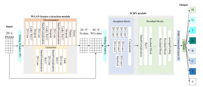
Protein secondary structure is the basis of studying the tertiary structure of proteins, drug design and development, and the 8-state protein secondary structure can provide more adequate protein information than the 3-state structure. Therefore, this paper proposes a novel method WG-ICRN for predicting protein 8-state secondary structures. First, we use the Wasserstein generative adversarial network (WGAN) to extract protein features in the position-specific scoring matrix (PSSM). The extracted features are combined with PSSM into a new feature set of WG-data, which contains richer feature information. Then, we use the residual network (ICRN) with Inception to further extract the features in WG-data and complete the prediction. Compared with the residual network, ICRN can reduce parameter calculations and increase the width of feature extraction to obtain more feature information. We evaluated the prediction performance of the model using six datasets. The experimental results show that the WGAN has excellent feature extraction capabilities, and ICRN can further improve network performance and improve prediction accuracy. Compared with four popular models, WG-ICRN achieves better prediction performance.
Citation: Shun Li, Lu Yuan, Yuming Ma, Yihui Liu. WG-ICRN: Protein 8-state secondary structure prediction based on Wasserstein generative adversarial networks and residual networks with Inception modules[J]. Mathematical Biosciences and Engineering, 2023, 20(5): 7721-7737. doi: 10.3934/mbe.2023333
Protein secondary structure is the basis of studying the tertiary structure of proteins, drug design and development, and the 8-state protein secondary structure can provide more adequate protein information than the 3-state structure. Therefore, this paper proposes a novel method WG-ICRN for predicting protein 8-state secondary structures. First, we use the Wasserstein generative adversarial network (WGAN) to extract protein features in the position-specific scoring matrix (PSSM). The extracted features are combined with PSSM into a new feature set of WG-data, which contains richer feature information. Then, we use the residual network (ICRN) with Inception to further extract the features in WG-data and complete the prediction. Compared with the residual network, ICRN can reduce parameter calculations and increase the width of feature extraction to obtain more feature information. We evaluated the prediction performance of the model using six datasets. The experimental results show that the WGAN has excellent feature extraction capabilities, and ICRN can further improve network performance and improve prediction accuracy. Compared with four popular models, WG-ICRN achieves better prediction performance.

| [1] |
A. W. Senior, R. Evans, J. Jumper, J. Kirkpatrick, L. Sifre, T. Green, et al., Improved protein structure prediction using potentials from deep learning, Nature, 577 (2020), 706–710. https://doi.org/10.1038/s41586-019-1923-7 doi: 10.1038/s41586-019-1923-7

|
| [2] |
J. Jumper, R. Evans, A. Pritzel, T. Green, M. Figurnov, O. Ronneberger, et al., Highly accurate protein structure prediction with AlphaFold, Nature, 596 (2021), 583–589. https://doi.org/10.1038/s41586-021-03819-2 doi: 10.1038/s41586-021-03819-2
|
| [3] | J. Zhou, O. Troyanskaya, Deep supervised and convolutional generative stochastic network for protein secondary structure prediction, in Proceedings of the 31st International Conference on Machine Learning (ICML-14), 32 (2014), 745–753. |
| [4] |
A. Yaseen, Y. H. Li, Template-based c8-scorpion: A protein 8-state secondary structure prediction method using structural information and context-based features, BMC Bioinformatics, 15 (2014). https://doi.org/10.1186/1471-2105-15-S8-S3 doi: 10.1186/1471-2105-15-S8-S3
|
| [5] | W. Kabsch, C. Sander, Dictionary of protein secondary structure, Biopolymers, 22 (1983), 2577–2637. |
| [6] |
B. Rost, C. Sander, Combining evolutionary information and neural networks to predict protein secondary structure, Proteins., 19 (1994), 55–72. https://doi.org/10.1002/prot.340190108 doi: 10.1002/prot.340190108
|
| [7] |
Y. Yang, J. Gao, J. Wang, R. Heffernan, J. Hanson, K. Paliwal, et al., Sixty-five years of the long march in protein secondary structure prediction: The final stretch?, Brief. Bioinform., 19 (2018), 482–494. https://doi.org/10.1093/bib/bbw129 doi: 10.1093/bib/bbw129
|
| [8] |
Y. Ma, Y. Liu, J. Cheng, Protein secondary structure prediction based on data partition and semi-random subspace method, Sci. Rep., 8 (2018), 1–10. https://doi.org/10.1038/s41598-018-28084-8 doi: 10.1038/s41598-018-28084-8
|
| [9] |
M. Lasfar, H. Bouden, A method of data mining using hidden markov models (HMMs) for protein secondary structure prediction, Procedia Comput. Sci., 127 (2018), 42–51. https://doi.org/10.1016/j.procs.2018.01.096 doi: 10.1016/j.procs.2018.01.096
|
| [10] |
A. Drozdetskiy, C. Cole, J. Procter, et al. JPred4: A protein secondary structure prediction server, Nucleic Acids Res., 43 (2015), 389–394. https://doi.org/10.1093/nar/gkv332 doi: 10.1093/nar/gkv332
|
| [11] |
D. T. Jones, Protein secondary structure prediction based on position-specific scoring matrices, J. Mol. Biol., 292 (1999), 195–202. https://doi.org/10.1006/jmbi.1999.3091 doi: 10.1006/jmbi.1999.3091
|
| [12] | A. Busia, N. Jaitly, Next-step conditioned deep convolutional neural networks improve protein secondary structure prediction, preprint, arXiv: 2017: 1702.0386. |
| [13] |
B. Z. Zhang, J. Y. Li, Q. Lü, Prediction of 8-state protein secondary structures by a novel deep learning architecture, BMC Bioinformatics, 19 (2018), 1–13. https://doi.org/10.1186/s12859-018-2280-5 doi: 10.1186/s12859-018-2280-5
|
| [14] |
S. Krieger, J. Kececioglu, Boosting the accuracy of protein secondary structure prediction through nearest neighbor search and method hybridization, Bioinformatics, 36 (2020). https://doi.org/10.1093/bioinformatics/btaa336 doi: 10.1093/bioinformatics/btaa336
|
| [15] |
M. R. Uddin, S. Mahbub, Saifur Rahman, M., Bayzid, M.S. SAINT: Self-attention augmented inception-inside-inception network improves protein secondary structure prediction, Bioinformatics, 36 (2020), 4599–4608. https://doi.org/10.1093/bioinformatics/btaa531 doi: 10.1093/bioinformatics/btaa531
|
| [16] |
K. Kotowski, T. Smolarczyk, I. Roterman-Konieczna, K. Stapor, ProteinUnet-An efficient alternative to SPIDER3-single for sequence-based prediction of protein secondary structures, J. Comput. Chem., 42 (2021), 50–59. https://doi.org/10.1002/jcc.26432 doi: 10.1002/jcc.26432
|
| [17] |
P. M. Sonsare, C. Gunavathi, Cascading 1D-convnet bidirectional long short term memory network with modified COCOB optimizer: A novel approach for protein secondary structure prediction, Chaos Soliton. Fract., 153 (2021), 111446. https://doi.org/10.1016/j.chaos.2021.111446 doi: 10.1016/j.chaos.2021.111446
|
| [18] | M. J. Zvelebil, J. O. Baum, Understanding Bioinformatics, Garland Science, New York, 2007. |
| [19] |
I. Goodfellow, J. Pouget-Abadie, M. Mirza, B. Xu, D. Warde-Farley, S. Ozair, et al., Generative adversarial networks, Commun. ACM, 63 (2020), 139–144. https://doi.org/10.1145/3422622 doi: 10.1145/3422622
|
| [20] |
R. Wang, X. Xiao, B. Guo, Q. Qin, R.Chen, An effective image denoising method for UAV images via improved generative adversarial networks, Sensors, 18 (2018), 1985. https://doi.org/10.3390/s18071985 doi: 10.3390/s18071985
|
| [21] | S. Yu, H. Chen, E. B. Garcia Reyes, N. Poh, Gaitgan: Invariant gait feature extraction using generative adversarial networks, in Proceedings of the IEEE Conference on Computer Vision and Pattern Recognition Workshops, 2017 (2017), 30–37. |
| [22] |
Y. Zhao, H. Zhang, Y. Liu, Protein secondary structure prediction based on generative confrontation and convolutional neural network, IEEE Access, 8 (2020), 199171–199178. https://doi.org/10.1109/ACCESS.2020.3035208 doi: 10.1109/ACCESS.2020.3035208
|
| [23] |
L. Abualigah, A. Diabat, S. Mirjalili, M. Abd Elaziz, A. H. Gandomi, The arithmetic optimization algorithm, Comput. Method. Appl. M., 376 (2021), 113609. https://doi.org/10.1016/j.cma.2020.113609 doi: 10.1016/j.cma.2020.113609
|
| [24] |
L. Abualigah, A. Diabat, P. Sumari, A. H. Gandomi, Applications, deployments, and integration of internet of drones (iod): A review, IEEE Sens. J., 21 (2021), 25532–25546. https://doi.org/10.1109/JSEN.2021.3114266 doi: 10.1109/JSEN.2021.3114266
|
| [25] |
L. Abualigah, M. Abd Elaziz, P. Sumari, Z. W. Geem, A. H. Gandomi, Reptile search algorithm (rsa): A nature-inspired meta-heuristic optimizer, Expert Syst. Appl., 191 (2022), 116158. https://doi.org/10.1016/j.eswa.2021.116158 doi: 10.1016/j.eswa.2021.116158
|
| [26] |
A. E. Ezugwu, J. O. Agushaka, L. Abualigah, S. Mirjalili, A. H. Gandomi, Prairie dog optimization algorithm, Neural Comput. Appl., 34 (2022), 20017–20065. https://doi.org/10.1007/s00521-022-07530-9 doi: 10.1007/s00521-022-07530-9
|
| [27] |
J. O. Agushaka, A. E. Ezugwu, L. Abualigah, Gazelle optimization algorithm: A novel nature-inspired metaheuristic optimizer, Neural Comput. Appl., 35 (2023), 4099–4131. https://doi.org/10.1007/s00521-022-07854-6 doi: 10.1007/s00521-022-07854-6
|
| [28] |
L. Abualigah, D. Yousri, M. Abd Elaziz, A. A. Ewees, M. A. Al-Qaness, A. H. Gandomi, Aquila optimizer: A novel meta-heuristic optimization algorithm, Comput. Ind. Eng., 157 (2021), 107250. https://doi.org/10.1016/j.cie.2021.107250 doi: 10.1016/j.cie.2021.107250
|
| [29] | M. Arjovsky, S. Chintala, L. Bottou, Wasserstein generative adversarial networks, in International Conference on Machine Learning, 70 (2017), 214–223. |
| [30] | K. He, X. Zhang, S. Ren, J. Sun, Deep residual learning for image recognition, in Proceedings of the IEEE Conference on Computer Vision and Pattern Recognition, (2016), 770–778. |
| [31] | M. Farooq, A. Hafeez, Covid-resnet: A deep learning framework for screening of covid19 from radiographs, preprint, arXiv: 2003.14395. |
| [32] |
Z. Wu, C. Shen, A. Van Den Hengel, Wider or deeper: Revisiting the resnet model for visual recognition, Pattern Recogn., 90 (2019), 119–133. https://doi.org/10.1016/j.patcog.2019.01.006 doi: 10.1016/j.patcog.2019.01.006
|
| [33] | K. He, X. Zhang, S. Ren, J. Sun, Identity mappings in deep residual networks, in European Conference on Computer Vision, Springer, Cham, (2016), 630–645. |
| [34] | C. Szegedy, W. Liu, Y. Jia, P. Sermanet, S. Reed, D. Anguelov, et al., Going deeper with convolutions, in Proceedings of the IEEE Conference on Computer Vision and Pattern Recognition, (2015), 1–9. |
| [35] |
G. Wang, R. L. Dunbrack, Pisces: Recent improvements to a PDB sequence culling server, Nucleic Acids Res., 33 (2005), W94–W98. https://doi.org/10.1093/nar/gki402 doi: 10.1093/nar/gki402
|
| [36] |
J. Moult, K. Fidelis, A. Kryshtafovych, T. Schwede, A. Tramontano, Critical assessment of methods of protein structure prediction (casp)-round x, Proteins., 82 (2014), 1–6. https://doi.org/10.1002/prot.24452 doi: 10.1002/prot.24452
|
| [37] |
J. Moult, K. Fidelis, A. Kryshtafovych, T. Schwede, A. Tramontano, Critical assessment of methods of protein structure prediction: Progress and new directions in round xi, Proteins., 84 (2016), 4–14. https://doi.org/10.1002/prot.25064 doi: 10.1002/prot.25064
|
| [38] |
J. Moult, K. Fidelis, A. Kryshtafovych, T. Schwede, A. Tramontano, Critical assessment of methods of protein structure prediction (casp)-round xii, Proteins., 86 (2018), 7–15. https://doi.org/10.1002/prot.25415 doi: 10.1002/prot.25415
|
| [39] |
A. Kryshtafovych, T. Schwede, M. Topf, K. Fidelis, J. Moult, Critical assessment of methods of protein structure prediction (casp)-round xiii, Proteins., 87 (2019), 1011–1020. https://doi.org/10.1002/prot.25823 doi: 10.1002/prot.25823
|
| [40] |
A. Kryshtafovych, T. Schwede, M. Topf, K. Fidelis, J. Moult, Critical assessment of methods of protein structure prediction (casp)-round xiv, Proteins., 89 (2021), 1607–1617. https://doi.org/10.1002/prot.26237 doi: 10.1002/prot.26237
|
| [41] | J. A. Cuff, G. J. Barton, Evaluation and improvement of multiple sequence methods for protein secondary structure prediction, Proteins., 34 (1999), 508–519. |
| [42] |
S. F. Altschul, T. L. Madden, A. A. Schäffer, J. Zhang, Z. Zhang, W. Miller et al., Gapped blast and psi-blast: a new generation of protein database search programs, Nucleic Acids Res., 25 (1997), 3389–3402. https://doi.org/10.1093/nar/25.17.3389 doi: 10.1093/nar/25.17.3389
|
| [43] |
B. Rost, C. Sander, R. Schneider, Redefining the goals of protein secondary structure prediction, J. Mol. Biol., 235 (1994), 13–26. https://doi.org/10.1016/S0022-2836(05)80007-5 doi: 10.1016/S0022-2836(05)80007-5
|
| [44] |
Y. Guo, W. Li, B. Wang, H. Liu, D. Zhou, Deepaclstm: Deep asymmetric convolutional long short-term memory neural models for protein secondary structure prediction, BMC bioinformatics, 20 (2019), 1–12. https://doi.org/10.1186/s12859-019-2940-0 doi: 10.1186/s12859-019-2940-0
|
| [45] |
A. R. Ratul, M. Turcotte, M. H. Mozaffari, W. S. Lee, Prediction of 8-state protein secondary structures by 1D-Inception and BD-LSTM, BioRxiv, 2019 (2019), 871921. https://doi.org/10.1101/871921 doi: 10.1101/871921
|
| [46] | Z. Li, Y. Yu, Protein secondary structure prediction using cascaded convolutional and recurrent neural networks, preprint, arXiv: 1604.07176. |
| [47] | I. Drori, I. Dwivedi, P. Shrestha, J. Wan, Y. Wang, Y. He, et al., High quality prediction of protein q8 secondary structure by diverse neural network architectures, preprint, arXiv: 1811.07143. |
Figures(9) / Tables(8)

Shun Li, Lu Yuan, Yuming Ma, Yihui Liu. WG-ICRN: Protein 8-state secondary structure prediction based on Wasserstein generative adversarial networks and residual networks with Inception modules[J]. Mathematical Biosciences and Engineering, 2023, 20(5): 7721-7737. doi: 10.3934/mbe.2023333


 DownLoad: