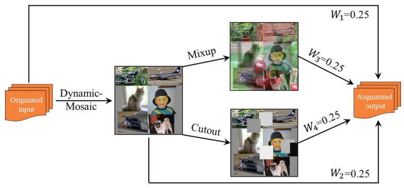
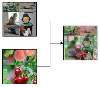
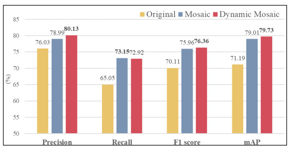
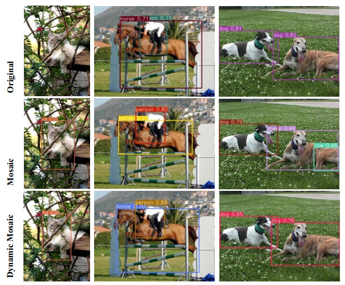
Convolutional Neural Networks (CNNs) have achieved remarkable results in the computer vision field. However, the newly proposed network architecture has deeper network layers and more parameters, which is more prone to overfitting, resulting in reduced recognition accuracy of the CNNs. To improve the recognition accuracy of the model of image recognition used in CNNs and overcome the problem of overfitting, this paper proposes an improved data augmentation approach based on mosaic algorithm, named Dynamic Mosaic algorithm, to solve the problem of the information waste caused by the gray background in mosaic images. This algorithm improves the original mosaic algorithm by adding a dynamic adjustment step that reduces the proportion of gray background in the mosaic image by dynamically increasing the number of spliced images. Moreover, to relieve the problem of network overfitting, also a Multi-Type Data Augmentation (MTDA) strategy, based on the Dynamic Mosaic algorithm, is introduced. The strategy divides the training samples into four parts, and each part uses different data augmentation operations to improve the information variance between the training samples, thereby preventing the network from overfitting. To evaluate the effectiveness of the Dynamic Mosaic algorithm and the MTDA strategy, we conducted a series of experiments on the Pascal VOC dataset and compared it with other state-of-the-art algorithms. The experimental results show that the Dynamic Mosaic algorithm and MTDA strategy can effectively improve the recognition accuracy of the model, and the recognition accuracy is better than other advanced algorithms.
Citation: Yuhua Li, Rui Cheng, Chunyu Zhang, Ming Chen, Hui Liang, Zicheng Wang. Dynamic Mosaic algorithm for data augmentation[J]. Mathematical Biosciences and Engineering, 2023, 20(4): 7193-7216. doi: 10.3934/mbe.2023311
Convolutional Neural Networks (CNNs) have achieved remarkable results in the computer vision field. However, the newly proposed network architecture has deeper network layers and more parameters, which is more prone to overfitting, resulting in reduced recognition accuracy of the CNNs. To improve the recognition accuracy of the model of image recognition used in CNNs and overcome the problem of overfitting, this paper proposes an improved data augmentation approach based on mosaic algorithm, named Dynamic Mosaic algorithm, to solve the problem of the information waste caused by the gray background in mosaic images. This algorithm improves the original mosaic algorithm by adding a dynamic adjustment step that reduces the proportion of gray background in the mosaic image by dynamically increasing the number of spliced images. Moreover, to relieve the problem of network overfitting, also a Multi-Type Data Augmentation (MTDA) strategy, based on the Dynamic Mosaic algorithm, is introduced. The strategy divides the training samples into four parts, and each part uses different data augmentation operations to improve the information variance between the training samples, thereby preventing the network from overfitting. To evaluate the effectiveness of the Dynamic Mosaic algorithm and the MTDA strategy, we conducted a series of experiments on the Pascal VOC dataset and compared it with other state-of-the-art algorithms. The experimental results show that the Dynamic Mosaic algorithm and MTDA strategy can effectively improve the recognition accuracy of the model, and the recognition accuracy is better than other advanced algorithms.

| [1] |
A. Belhadi, Y. Djenouri, G. Srivastava, D. Djenouri, J. C. W. Lin, G. Fortino, Deep learning for pedestrian collective behavior analysis in smart cities: a model of group trajectory outlier detection, Inform. Fusion, 65 (2021), 13–20. https://doi.org/10.1016/j.inffus.2020.08.003 doi: 10.1016/j.inffus.2020.08.003

|
| [2] |
G. Vallathan, A. John, C. Thirumalai, S. K. Mohan, G. Srivastava, J. C. W. Lin, Suspicious activity detection using deep learning in secure assisted living IoT environments, J. supercomput., 77 (2021), 3242–3260. https://doi.org/10.1007/s11227-020-03387-8 doi: 10.1007/s11227-020-03387-8
|
| [3] |
Y. Djenouri, G. Srivastava, J. C. W. Lin, Fast and accurate convolution neural network for detecting manufacturing data, IEEE Trans. Ind. Inform., 17 (2020), 2947–2955. https://doi.org/10.1109/TII.2020.3001493 doi: 10.1109/TII.2020.3001493
|
| [4] |
A. Belhadi, Y. Djenouri, J. C. W. Lin, A. Cano, Trajectory outlier detection: algorithms, taxonomies, evaluation and open challenges, ACM Trans. Manage. Inform. Syst., 11 (2020), 1–29. https://doi.org/10.1145/3399631 doi: 10.1145/3399631
|
| [5] |
A. Belhadi, Y. Djenouri, G. Srivastava, D. Djenouri, A. Cano, J. C. W. Lin, A two-phase anomaly detection model for secure intelligent transportation ride-hailing trajectories, IEEE Trans. Intell. Trans. Syst., 22 (2020), 4496–4506. https://doi.org/10.1109/TITS.2020.3022612 doi: 10.1109/TITS.2020.3022612
|
| [6] | C. Sun, A. Shrivastava, S. Singh, A. Gupta, Revisiting unreasonable effectiveness of data in deep learning era, in Proceedings of the IEEE international conference on computer vision, (2017), 843–852. https://doi.org/10.1109/ICCV.2017.97 |
| [7] |
R. Takahashi, T. Matsubara, K. Uehara, Data augmentation using random image cropping and patching for deep CNNs, IEEE Trans. Circuits Syst. Video Technol., 30 (2019), 2917–2931. https://doi.org/10.1109/TCSVT.2019.2935128 doi: 10.1109/TCSVT.2019.2935128
|
| [8] |
C. Zhang, S. Bengio, M. Hardt, B. Recht, O. Vinyals, Understanding deep learning (still) requires rethinking generalization, Commun. ACM, 64 (2021), 107–115. https://doi.org/10.1145/3446776 doi: 10.1145/3446776
|
| [9] | M. D. Zeiler, R. Fergus, Visualizing and understanding convolutional networks. in European conference on computer vision, (2014), 818–833. https://doi.org/10.1007/978-3-319-10590-1_53 |
| [10] | L. M. Zintgraf, T. S. Cohen, T. Adel, M. Welling, Visualizing deep neural network decisions: Prediction difference analysis, preprint, arXiv: 1702.04595. |
| [11] |
L. Schmidt, S. Santurka, D. Tsipras, K. Talwar, A. Madry, Adversarially robust generalization requires more data, Adv. Neural Inform. Process. Syst., 31 (2018). https://doi.org/10.48550/arXiv.1804.11285 doi: 10.48550/arXiv.1804.11285
|
| [12] | J. Hestness, S. Narang, N. Ardalani, G. Diamos, H. Jun, H. Kianinejad, et al., Deep learning scaling is predictable, preprint, arXiv: 1712.00409. |
| [13] | D. C. Ciresan, U. Meier, J. Masci, L. M. Gambardella, J. Schmidhuber, Flexible, high performance convolutional neural networks for image classification, in Twenty-second international joint conference on artificial intelligence, (2011), 1237–1242. |
| [14] | D. Cireşan, U. Meier, J. Schmidhuber, Multi-column deep neural networks for image classification, in IEEE conference on computer vision and pattern recognition, (2012), 3642–3649. https://doi.org/10.1109/CVPR.2012.6248110 |
| [15] |
C. Shorten, T. M. Khoshgoftaar, A survey on image data augmentation for deep learning, J. Big Data, 6 (2019), 1–48. https://doi.org/10.1186/s40537-019-0197-0 doi: 10.1186/s40537-018-0162-3
|
| [16] | D. Han, J. Kim, J. Kim, Deep pyramidal residual networks. in Proceedings of the IEEE conference on computer vision and pattern recognition, (2017), 5927–5935. https://doi.org/10.1109/cvpr.2017.668 |
| [17] |
A. Krizhevsky, I. Sutskever, G. E. Hinton, Imagenet classification with deep convolutional neural networks, Adv. Neural Inform. Process. Syst., 6 (2017), 84–90. https://doi.org/10.1145/3065386 doi: 10.1145/3065386
|
| [18] | K. Simonyan, A. Zisserman, Very deep convolutional networks for large-scale image recognition, preprint, arXiv: 1409.1556. |
| [19] | K. He, X. Zhang, S. Ren, J. Sun, Deep residual learning for image recognition, in Proceedings of the IEEE conference on computer vision and pattern recognition, (2016), 770–778. |
| [20] | G. Huang, Z. Liu, L. Van Der Maaten, K. Q. Weinberger, Densely connected convolutional networks, in Proceedings of the IEEE conference on computer vision and pattern recognition, (2017), 4700–4708 |
| [21] | S. Xie, R. Girshick, P. Dollár, Z. Tu, K. He, Aggregated residual transformations for deep neural networks, in Proceedings of the IEEE conference on computer vision and pattern recognition, (2017), 1492–1500. https://doi.org/10.1109/CVPR.2017.634 |
| [22] | Y. Tokozume, Y. Ushiku, T. Harada, Between-class learning for image classification, in Proceedings of the IEEE Conference on Computer Vision and Pattern Recognition, (2018), 5486–5494. https://doi.org/10.48550/arXiv.1711.10284 |
| [23] | A. Bochkovskiy, C. Y. Wang, H. Y. M. Liao, Yolov4: Optimal speed and accuracy of object detection, preprint, arXiv: 2004.10934. |
| [24] | S. Ioffe, C. Szegedy, Batch normalization: Accelerating deep network training by reducing internal covariate shift, in International conference on machine learning PMLR, (2015), 448–456. |
| [25] | J. Kukačka, V. Golkov, D. Cremers, Regularization for deep learning: A taxonomy, preprint, arXiv: 1710.10686. |
| [26] | J. Niu, Y. Chen, X. Yu, Z. Li, H. Gao, Data augmentation on defect detection of sanitary ceramics, in IECON The 46th Annual Conference of the IEEE Industrial Electronics Society, (2020), 5317–5322. https://doi.org/10.1109/IECON43393.2020.9254518 |
| [27] | A. Jurio, M. Pagola, M. Galar, C. Lopez-Molina, D. Paternain, A comparison study of different color spaces in clustering based image segmentation, in International conference on information processing and management of uncertainty in knowledge-based systems, (2020), 532–541. https://doi.org/10.1007/978-3-642-14058-7_55 |
| [28] | A. Krizhevsky, G. Hinton, Learning multiple layers of features from tiny images, Handb. Syst. Autoimmune Dis., 2009. |
| [29] | F. J. Moreno-Barea, F. Strazzera, J. M. Jerez, D. Urda, L. Franco, Forward noise adjustment scheme for data augmentation, in IEEE symposium series on computational intelligence (SSCI), (2018), 728–734. https://doi.org/10.1109/SSCI.2018.8628917 |
| [30] | T. DeVries, G. W. Taylor, Improved regularization of convolutional neural networks with cutout, 2017, preprint, arXiv: 1708.04552. |
| [31] | E. D. Cubuk, B. Zoph, D. Mane, V. Vasudevan, Q. V. Le, Autoaugment: Learning augmentation policies from data, preprint, arXiv: 1805.09501. |
| [32] |
J. Gui, Z. Sun, Y. Wen, D. Tao, J. Ye, A review on generative adversarial networks: Algorithms, theory, and applications, IEEE Trans. Knowl. Data Eng., 2021. https://doi.org/10.1109/TKDE.2021.3130191 doi: 10.1109/TKDE.2021.3130191
|
| [33] | D. Ho, E. Liang, X. Chen, I. Stoica, P. Abbeel, Population based augmentation: Efficient learning of augmentation policy schedules, in International Conference on Machine Learning, (2019), 2731–2741. https://doi.org/10.48550/arXiv.1905.05393 |
| [34] | S. Lim, I. Kim, T. Kim, C. Kim, S. Kim, Fast autoaugment, Adv. Neural Inform. Process. Syst., 32 (2019). |
| [35] | M. Frid-Adar, E. Klang, M. Amitai, J. Goldberger, H. Greenspan, Synthetic data augmentation using GAN for improved liver lesion classification, in IEEE 15th international symposium on biomedical imaging (ISBI), (2018), 289–293. https://doi.org/10.1109/ISBI.2018.8363576 |
| [36] | A. Raghunathan, S. M. Xie, F. Yang, J. C. Duchi, P. Liang, Adversarial training can hurt generalization, preprint, arXiv: 1906.06032. |
| [37] | H. Zhang, M. Cisse, Y. N. Dauphin, D. Lopez-Paz, mixup: Beyond empirical risk minimization, 2017, preprint, arXiv: 1710.09412. |
| [38] | R. Takahashi, T. Matsubara, K. Uehara, Ricap: Random image cropping and patching data augmentation for deep cnns, in Asian conference on machine learning, (2018), 786–798. |
| [39] | H. Guo, Y. Mao, R. Zhang, Mixup as locally linear out-of-manifold regularization, in Proceedings of the AAAI Conference on Artificial Intelligence, 33 (2019), 3714–3722. https://doi.org/10.48550/arXiv.1809.02499 |
| [40] | S.Yun, D. Han, S. J. Oh, S. Chun, J. Choe, Y. Yoo, Cutmix: Regularization strategy to train strong classifiers with localizable features, in Proceedings of the IEEE/CVF international conference on computer vision, (2019), 6023–6032. |
| [41] | C. Summers, M. J. Dinneen, Improved mixed-example data augmentation, in IEEE Winter Conference on Applications of Computer Vision (WACV), (2019), 1262–1270. |
| [42] |
M. Everingham, S. M. Eslami, L. Van Gool, C. K. Williams, J. Winn, A. Zisserman, The pascal visual object classes challenge: A retrospective, Int. J. Comput. Vision, 111 (2015), 98–136. https://doi.org/10.1007/s11263-014-0733-5 doi: 10.1007/s11263-014-0733-5
|
| [43] | J. Glenn, S. Alex, B. Jirka, ultralytics/yolov5: v5.0 – YOLOv5 -P6 1280 models, 2021. Available from: https://github.com/ultralytics/yolov5. |
| [44] | I. Loshchilov, F. Hutter, Sgdr: Stochastic gradient descent with warm restarts, preprint, arXiv: 1608.03983. |
| [45] | W. Hao, S. Zhili, Improved mosaic: Algorithms for more complex images, in Journal of Physics: Conference Series, 1684 (2020), 012094. https://doi.org/10.1088/1742-6596/1684/1/012094 |
Figures(10) / Tables(8)

Yuhua Li, Rui Cheng, Chunyu Zhang, Ming Chen, Hui Liang, Zicheng Wang. Dynamic Mosaic algorithm for data augmentation[J]. Mathematical Biosciences and Engineering, 2023, 20(4): 7193-7216. doi: 10.3934/mbe.2023311


 DownLoad: