


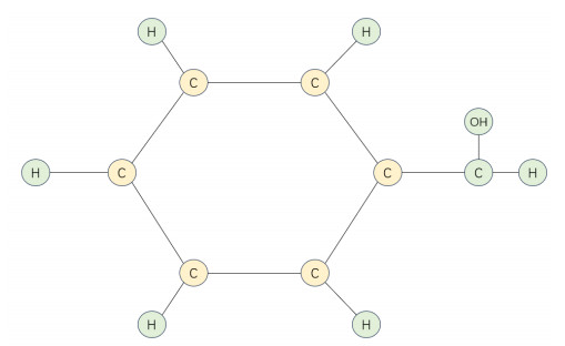
Figure 1.
Molecular structure of benzoic acid.
Citation: Robert Carlson. Spectral theory for nonconservative transmission line networks[J]. Networks and Heterogeneous Media, 2011, 6(2): 257-277. doi: 10.3934/nhm.2011.6.257
| [1] | Khaled M. Bataineh, Assem N. AL-Karasneh . Direct solar steam generation inside evacuated tube absorber. AIMS Energy, 2016, 4(6): 921-935. doi: 10.3934/energy.2016.6.921 |
| [2] | Sunbong Lee, Shaku Tei, Kunio Yoshikawa . Properties of chicken manure pyrolysis bio-oil blended with diesel and its combustion characteristics in RCEM, Rapid Compression and Expansion Machine. AIMS Energy, 2014, 2(3): 210-218. doi: 10.3934/energy.2014.3.210 |
| [3] | Saad S. Alrwashdeh . Investigation of the effect of the injection pressure on the direct-ignition diesel engine performance. AIMS Energy, 2022, 10(2): 340-355. doi: 10.3934/energy.2022018 |
| [4] | Xiaoyu Zheng, Dewang Chen, Yusheng Wang, Liping Zhuang . Remaining useful life indirect prediction of lithium-ion batteries using CNN-BiGRU fusion model and TPE optimization. AIMS Energy, 2023, 11(5): 896-917. doi: 10.3934/energy.2023043 |
| [5] | Gitsuzo B.S. Tagawa, François Morency, Héloïse Beaugendre . CFD investigation on the maximum lift coefficient degradation of rough airfoils. AIMS Energy, 2021, 9(2): 305-325. doi: 10.3934/energy.2021016 |
| [6] | Charalambos Chasos, George Karagiorgis, Chris Christodoulou . Technical and Feasibility Analysis of Gasoline and Natural Gas Fuelled Vehicles. AIMS Energy, 2014, 2(1): 71-88. doi: 10.3934/energy.2014.1.71 |
| [7] | Tien Duy Nguyen, Trung Tran Anh, Vinh Tran Quang, Huy Bui Nhat, Vinh Nguyen Duy . An experimental evaluation of engine performance and emissions characteristics of a modified direct injection diesel engine operated in RCCI mode. AIMS Energy, 2020, 8(6): 1069-1087. doi: 10.3934/energy.2020.6.1069 |
| [8] | Abdelrahman Kandil, Samir Khaled, Taher Elfakharany . Prediction of the equivalent circulation density using machine learning algorithms based on real-time data. AIMS Energy, 2023, 11(3): 425-453. doi: 10.3934/energy.2023023 |
| [9] | Anbazhagan Geetha, S. Usha, J. Santhakumar, Surender Reddy Salkuti . Forecasting of energy consumption rate and battery stress under real-world traffic conditions using ANN model with different learning algorithms. AIMS Energy, 2025, 13(1): 125-146. doi: 10.3934/energy.2025005 |
| [10] | Kunzhan Li, Fengyong Li, Baonan Wang, Meijing Shan . False data injection attack sample generation using an adversarial attention-diffusion model in smart grids. AIMS Energy, 2024, 12(6): 1271-1293. doi: 10.3934/energy.2024058 |
Fractional calculus is a branch of mathematics that investigates the properties of arbitrary-order differential and integral operators to address various problems. Fractional differential equations provide a more appropriate model for describing diffusion processes, wave phenomena, and memory effects [1,2,3,4] and possess a diverse array of applications across numerous fields, encompassing stochastic equations, fluid flow, dynamical systems theory, biological and chemical engineering, and other domains[5,6,7,8,9].
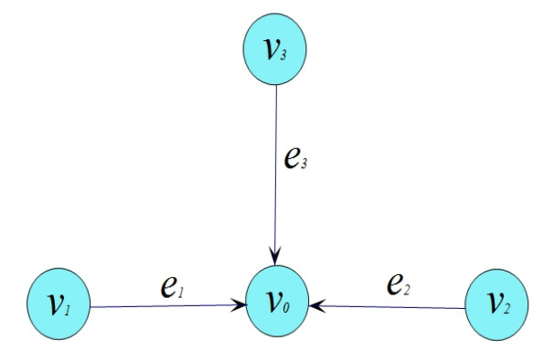
Star graph $ G = (V, E) $ consists of a finite set of nodes or vertices $ V(G) = \{v_{0}, v_{1}, ..., v_{k}\} $ and a set of edges $ E(G) = \{e_{1} = \overrightarrow{v_{1}v_{0}}, e_{2} = \overrightarrow{v_{2}v_{0}}, ..., e_{k} = \overrightarrow{v_{k}v_{0}}\} $ connecting these nodes, where $ v_{0} $ is the joint point and $ e_{i} $ is the length of $ l_{i} $ the edge connecting the nodes $ v_{i} $ and $ v_{0} $, i.e., $ l_{i} = |\overrightarrow{v_{i}v_{0}}| $.
Graph theory is a mathematical discipline that investigates graphs and networks. It is frequently regarded as a branch of combinatorial mathematics. Graph theory has become widely applied in sociology, traffic management, telecommunications, and other fields[10,11,12].
Differential equations on star graphs can be applied to different fields, such as chemistry, bioengineering, and so on[13,14]. Mehandiratta et al. [15] explored the fractional differential system on star graphs with $ n+1 $ nodes and $ n $ edges,
| $ {CDα0,xui(x)=fi(x,ui,CDβ0,xui(x)),0<x<li,i=1,2,...,k,ui(0)=0,i=1,2,...,k,ui(li)=uj(lj),i,j=1,2,...,k,i≠j,k∑i=1u′i=0,i=1,2,...,k, $ |
where $ {}^{C}D^{\alpha}_{0, x}, \; {}^{C}D^{\beta}_{0, x} $ are the Caputo fractional derivative operator, $ 1 < \alpha\leq2 $, $ 0 < \beta\leq\alpha-1 $, $ \mathfrak{f}_{i}, i = 1, 2, ..., k $ are continuous functions on $ C([0, 1]\times\mathbb R\times\mathbb R) $. By a transformation, the equivalent fractional differential system defined on $ [0, 1] $ is obtained. The author studied a nonlinear Caputo fractional boundary value problem on star graphs and established the existence and uniqueness results by fixed point theory.
Zhang et al. [16] added a function $ \lambda_{i}(x) $ on the basis of the reference [15]. In addition, Wang et al. [17] discussed the existence and stability of a fractional differential equation with Hadamard derivative. For more papers on the existence of solutions to fractional differential equations, refer to [18,19,20,21]. By numerically simulating the solution of fractional differential systems, we are able to solve problems more clearly and accurately. However, numerical simulation has been rarely used to describe the solutions of fractional differential systems on graphs [22,23].
The word chemical is used to distinguish chemical graph theory from traditional graph theory, where rigorous mathematical proofs are often preferred to the intuitive grasp of key ideas and theorems. However, graph theory is used to represent the structural features of chemical substances. Here, we introduce a novel modeling of fractional boundary value problems on the benzoic acid graph (Figure 1). The molecular structure of the benzoic acid seven carbon atoms, seven hydrogen atoms, and one oxygen atom. Benzoic acid is mainly used in the preparation of sodium benzoate preservatives, as well as in the synthesis of drugs and dyes. It is also used in the production of mordants, fungicides, and fragrances. Therefore, a thorough understanding of its properties is of utmost importance.
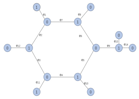
By this structure, we consider atoms of carbon, hydrogen, and oxygen as the vertices of the graph and also the existing chemical bonds between atoms are considered as edges of the graph. To investigate the existence of solutions for our fractional boundary value problems, we label vertices of the benzoic acid graph in the form of labeled vertices by two values, 0 or 1, and the length of each edge is fixed at $ e $ ($ |\overrightarrow{e_{i}}| = e, \; i = 1, 2, ..., 14 $) (Figure 2). In this case, we construct a local coordinate system on the benzoic acid graph, and the orientation of each vertex is determined by the orientation of its corresponding edge. The labels of the beginning and ending vertices are taken into account as values 0 and 1, respectively, as we move along any edge.
Motivated by the above work and relevant literature[15,16,17,18,19,20,21,22,23], we discuss a boundary value problem consisting of nonlinear fractional differential equations defined on $ |\overrightarrow{e_{i}}| = e, \; i = 1, 2, \cdots, 14 $ by
| $ {}^{H}D^{\alpha}_{1^{+}} r_{i}(t) = -\varrho_{i}^{\alpha}\phi_{p}\left(f_{i}\big(s,r_{i}(s),{}^{H}D^{\beta}_{1^{+}}r_{i}(s)\big)\right),\; t \in [1,e], $ |
and the boundary conditions defined at boundary nodes $ e_{1}, e_{2}, \cdots, e_{14} $, and
| $ r_{i}(1) = 0,r_{i}(e) = r_{j}(e),\; i,j = 1,2,\cdots,14,\; i\neq j, $ |
together with conditions of conjunctions at 0 or 1 with
| $ \sum\limits_{i = 1}^{k}\varrho_{i}^{-1}r'_{i}(e) = 0,\; i = 1,2,\cdots,14. $ |
Overall, we consider the existence and stability of solutions to the following nonlinear boundary value problem on benzoic acid graphs:
| $ {HDα1+ri(t)=−ϱαiϕp(fi(s,ri(s),HDβ1+ri(s))),t∈[1,e],ri(1)=0,i=1,2,⋯,14,ri(e)=rj(e),i,j=1,2,⋯,14,i≠j,k∑i=1ϱ−1ir′i(e)=0,i=1,2,⋯,14, $ | (1.1) |
where $ {}^{H}D^{\alpha}_{1^{+}}, {}^{H}D^{\beta}_{1^{+}} $ represent the Hadamard fractional derivative, $ \alpha\in (1, 2], \; \beta\in (0, 1], \; f_{i}\in C([1, e]\times\mathbb R \times\mathbb R) $, $ \varrho_{i} $ is a real constant, and $ \phi_{p}(s) = sgn(s)\cdot |s|^{p-1} $. The existence and Hyers-Ulam stability of the solutions to the system (1.1) are discussed. Moreover, the approximate graphs of the solution are obtained.
It is also noteworthy that solutions obtained from the problem (1.1) can be depicted in various rational applications of organic chemistry. More precisely, any solution on an arbitrary edge can be described as the amount of bond polarity, bond power, bond energy, etc. This paper lies in the integration of fractional differential equations with graph theory, utilizing the formaldehyde graph as a specific case for numerical simulation, and providing an approximate solution graph after iterations.
In this section, for conveniently researching the problem, several properties and lemmas of fractional calculus are given, forming the indispensable premises for obtaining the main conclusions.
Definition 2.1. [2,20] The Hadamard fractional integral of order $ \alpha $, for a function $ g\in L^{p}[a, b] $, $ 0\leq a\leq t\leq b \leq \infty $, is defined as
| $ {}^{H}I^{q}_{a^+}g(t) = \frac{1}{\Gamma(\alpha)} \int_{a}^{t}\left(\log\frac{t}{s}\right)^{\alpha-1}\frac{g(s)}{s}ds, $ |
and the Hadamard fractional integral is a particular case of the generalized Hattaf fractional integral introduced in [24].
Definition 2.2. [2,20] Let $ [a, b]\subset\mathbb R $, $ \delta = t\frac{d}{dt} $ and $ AC^{n}_{\delta}[a, b] = \{g:[a, b]\rightarrow \mathbb R:\delta^{n-1}(g(t))\in AC[a, b]\}. $ The Hadamard derivative of fractional order $ \alpha $ for a function $ g\in AC^{n}_{\delta} [a, b] $ is defined as
| $ {}^{H}D_{a^+}^{\alpha}g(t) = \delta^{n} ({}^{H}I^{n-\alpha}_{a^+})(t) = \frac{1}{\Gamma(n-\alpha)}\Big(t\frac{d}{dt}\Big)^{n} \int_{a}^{t}\left(\log\frac{t}{s}\right)^{n-\alpha-1} \frac{g(s)}{s}ds, $ |
where $ n-1 < \alpha < n $, $ n = [\alpha]+1 $, and $ [\alpha] $ denotes the integer part of the real number $ \alpha $ and $ log(\cdot) = log_{e}(\cdot) $.
Definition 2.3. [25] Completely continuous operator: A bounded linear operator $ f $, acting from a Banach space $ X $ into another space $ Y $, that transforms weakly-convergent sequences in $ X $ to norm-convergent sequences in $ Y $. Equivalently, an operator $ f $ is completely-continuous if it maps every relatively weakly compact subset of $ X $ into a relatively compact subset of $ Y $.
Compact operator: An operator $ A $ defined on a subset $ M $ of a topological vector space $ X $, with values in a topological vector space $ Y $, such that every bounded subset of $ M $ is mapped by it into a pre-compact subset of $ Y $. If, in addition, the operator $ A $ is continuous on $ M $, then it is called completely continuous on this set. In the case when $ X $ and $ Y $ are Banach or, more generally, bornological spaces and the operator $ A:X\rightarrow Y $ is linear, the concepts of a compact operator and of a completely-continuous operator are the same.
Lemma 2.4. [20] For $ y\in AC^{n}_{\delta}[a, b] $, the following result hold
| $ ^{H}I_{0^{+}}^{\alpha}(^{H}D_{0^{+}}^{\alpha})y(t) = y(t)- \sum\limits_{k = 0}^{n-1}c_{i}\left(\log\frac{t}{a}\right)^{k}, $ |
where $ c_{i}\in \mathbb{\mathbb{R}}, \; i = 0, 1, \cdots, n-1 $.
Lemma 2.5. [21] For $ p > 2 $, $ \mid x\mid, \; \mid y\mid\leq M $, we have
| $ \mid\phi_{p}(x)-\phi_{p}(y)\mid\leq(p-1)M^{p-2}\mid x-y\mid. $ |
Lemma 2.6. [4] Let $ M $ be a closed convex and nonempty subset of a Banach space $ X $. Let $ T, S $ be the operators $ T-S:M\rightarrow X $ such that
(ⅰ) $ Tx+Sy\in M $ whenever $ x, y\in M $;
(ⅱ) $ T $ is contraction mapping;
(ⅲ) $ S $ is completely continuous in $ M $.
Then $ T+S $ has at least one fixed point in $ M $.
Proof. For every $ Z\in S(M) $, we have $ T(x)+z:M\rightarrow M $. According to (ⅱ) and the Banach contraction mapping principle, $ Tx+z = x $ or $ z-x = Tx $ has only one solution in $ M $. For any $ z, \tilde{z}\in S(M) $, we have
| $ T(t(z))+z = T(z), T(t(\tilde{z}))+z = t(\tilde{z}). $ |
So we have
| $ |t(z)-t(\tilde{z})|\leq|T(t(z))-T(t(\tilde{z}))|+|z-\tilde{z}|\leq \nu|t(z)-t(\tilde{z})|+|z-\tilde{z}|, 0\leq\nu < 1. $ |
Thus, $ |t(z)-t(\tilde{z})|\leq \frac{1}{1-\nu}|z-\tilde{z}| $. It indicates that $ t\in C(S(M)) $. Because of $ S $ is completely continuous in $ M $, $ tS $ is completely continuous. According to the Schauder fixed point theorem, there exists $ x^{\ast}\in M $, such that $ tS(x^{\ast}) = x $. So we have
| $ T(t(S(x^{\ast})))+S(x^{\ast}) = t(S(x^{\ast})), Tx^{\ast}+Sx^{\ast} = x^{\ast}. $ |
Lemma 2.7. Let $ h_{i}(t)\in AC([1, e], \mathbb R), \; i = 1, 2, \cdots, 14 $; then the solution of the fractional differential equations
| $ {HDα1+ri(t)=−ζi(t),t∈[1,e],ri(1)=0,i=1,2,⋯,14,ri(e)=rj(e),i,j=1,2,⋯,14,i≠j,k∑i=1ϱ−1ir′i(e)=0,i=1,2,⋯,14, $ | (2.1) |
is given by
| $ ri(t)=−1Γ(α)∫t1(logts)α−1ζi(s)sds +logt[1Γ(α−1)k∑j=1(ϱ−1j∑kj=1ϱ−1j)∫e1(loges)α−2ζj(s)sds −1Γ(α)k∑j=1j≠i(ϱ−1j∑kj=1ϱ−1j)(∫e1(loges)α−1(ζj(s)−ζi(s)s))ds]. $ | (2.2) |
Proof. By Lemma 2.4, we have
| $ r_{i}(t) = -{}^{H}I_{1^{+}}^{\alpha}\zeta_{i}(t)+c_{i}^{(1)}+c_{i}^{(2)}\log t,\; i = 1,2,\cdots,14, $ |
where $ c_{i}^{(1)}, \; c_{i}^{(2)} $ are constants. The boundary condition $ r_{i}(1) = 0 $ gives $ c_{i}^{(1)} = 0, $ for $ i = 1, 2, \cdots, 14. $
Hence,
| $ ri(t)=−HIα1+ζi(t)+c(2)ilogt =−1Γ(α)∫t1(logts)α−1ζ(s)sds+c(2)ilogt,i=1,2,⋯,14. $ | (2.3) |
Also
| $ r'_{i}(t) = -\frac{1}{\Gamma(\alpha-1)} \int_{1}^{t}\frac{1}{t}\Big(\log\frac{t}{s}\Big)^{\alpha-2}\frac{\zeta(s)}{s}ds+\frac{1}{t}c_{i}^{(2)}. $ |
Now, the boundary conditions $ r_{i}(e) = r_{j}(e) $ and $ \sum\limits_{i = 1}^{k}\varrho_{i}^{-1}r'_{i}(e) = 0 $ implies that $ c_{i}^{(2)} $ must satisfy
| $ −1Γ(α)∫e1(loges)α−1ζi(s)sds+c(2)i=−1Γ(α)∫e1(loges)α−1ζj(s)sds+c(2)j, $ | (2.4) |
| $ −k∑i=1ϱ−1i(1Γ(α−1)∫e1(loges)α−2ζi(s)sds−c(2)i)=0. $ | (2.5) |
On solving above Eqs (2.4) and (2.5), we have
| $ −k∑j=1ϱ−1j(1Γ(α−1)∫e1(loges)α−2ζj(s)sds)+λ−1ic(2)i=−k∑j=1j≠iϱ−1j[1Γ(α)∫e1(loges)α−1ζj(s)sds−1Γ(α)∫e1(loges)α−1ζi(s)sds+c(2)i], $ |
which implies
| $ k∑j=1ϱ−1jc(2)i=−k∑j=1ϱ−1j1Γ(α−1)∫e1(loges)α−2ζj(s)sds+k∑j=1j≠iϱ−1j1Γ(α)∫e1(loges)α−1(ζj(s)−ζi(s)s)ds. $ |
Hence, we get
| $ c(2)i=−1Γ(α−1)k∑j=1(ϱ−1j∑kj=1ϱ−1j)∫e1(loges)α−2ζj(s)sds +1Γ(α)k∑j=1j≠i(ϱ−1j∑kj=1ϱ−1j)(∫e1(loges)α−1(ζj(s)−ζi(s)s))ds. $ | (2.6) |
Hence, inserting the values of $ c_{i}^{(2)} $, we get the solution (2.2). This completes the proof.
In this section, we discuss the existence and uniqueness of solutions of system (1.1) by using fixed point theory.
We define the space $ X = \{r:r\in C([1, e], \mathbb R), {}^{H}D^{\beta}_{1^{+}}r\in C([1, e], \mathbb R)\} $ with the norm
| $ \|r\|_{X} = \|r\|+\left\|^{H}D^{\beta}_{1^{+}}u\right\| = \sup\limits_{t\in[1,e]}|r(t)|+ \sup\limits_{t\in[1,e]}\left|^{H}D^{\beta}_{1^{+}}r(t)\right|. $ |
Then, $ (X, \|.\|_{X}) $ is a Banach space, and accordingly, the product space $ \big(X^{k} = X_{1}\times X_{2}\cdots\times X_{14}, \; \|.\|_{X^{k}}\big) $ is a Banach space with norm
| $ \|r\|_{X^{k}} = \|(r_{1},r_{2},\cdots,r_{14})\|_{X} = \sum\limits_{\substack{i = 1}}^{k}\|r_{i}\|_{X},\; (r_{1},r_{2},\cdots,r_{k})\in X^{k}. $ |
In view of Lemma 2.7, we define the operator $ T:X^{k}\rightarrow X^{k} $ by
| $ T(r_{1},r_{2},\cdots, r_{k})(t): = \left(T_{1}(r_{1},r_{2},\cdots, r_{k})(t),\cdots, T_{k}(r_{1},r_{2},\cdots, r_{k})(t)\right), $ |
where
| $ Ti(r1,r2,⋯,rk)(t)=−ϱαiΓ(α)∫t1(logts)α−1ϕp(gi(s,ri(s),HDβ1+ri(s)))ds+logtΓ(α−1)k∑j=1(ϱ−1j∑kj=1ϱ−1j)ϱαj∫e1(loges)α−2ϕp(gj(s,rj(s),HDβ1+rj(s)))ds−logtΓ(α)k∑j=1j≠i(ϱ−1j∑kj=1ϱ−1j)ϱαj∫e1(loges)α−1ϕp(gj(s,rj(s),HDβ1+rj(s)))ds+logtΓ(α)k∑j=1j≠i(ϱ−1j∑kj=1ϱ−1j)ϱαi∫e1(loges)α−1ϕp(gi(s,ri(s),HDβ1+ri(s)))ds, $ | (3.1) |
where $ \phi_{p}\left(\frac{f_{i}\big(s, r_{i}(s), {}^{H}D^{\beta}_{1^{+}}r_{i}(s)\big)}{s}\right) = \phi_{p}\left(g_{i}\big(s, r_{i}(s), {}^{H}D^{\beta}_{1^{+}}r_{i}(s)\big)\right) $.
Assume that the following conditions hold:
$ (H_{1}) $ $ g_{i}:[1, e]\times\mathbb R\times\mathbb R\rightarrow \mathbb R, i = 1, 2, \cdots, 14 $ be continuous functions, and there exists nonnegative functions $ l_{i}(t)\in C[1, e] $ such that
| $ \left|g_{i}(t,x,y)-g_{i}(t,x_{1},y_{1})\right|\leq u_{i}(t)(|x-x_{1}|+|y-y_{1}|), $ |
where $ t\in[1, e], (x, y), (x_{1}, y_{1})\in\mathbb R^{2}; $
$ (H_{2}) $ $ \iota_{i} = \sup\limits_{t\in [1, e]}|u_{i}(t)|, \; i = 1, 2, \cdots, 14; $
$ (H_{3}) $ There exists $ Q_{i} > 0 $, such that
| $ |g_{i}(t,x,y)|\leq Q_{i},\; t\in [1,e],\; (x,y)\in\mathbb R\times\mathbb R,\; i = 1,2,\cdots,14; $ |
$ (H_{4})\; \sup\limits_{1\leq t\leq e}\mid g_{i}(t, 0, 0)\mid = \kappa < \infty, \; i = 1, 2, ..., 14 $.
For computational convenience, we also set the following quantities:
| $ χi=e(p−1)Qp−2i(ϱαi+ϱα−βi) ×[1Γ(α)+2Γ(α+1)+1Γ(α−β+1)+1Γ(α)Γ(2−β)+1Γ(α+1)Γ(2−β)] +ek∑j=1j≠i(ϱαj+ϱα−βj)(p−1)Qp−2j ×[1Γ(α)+1Γ(α+1)+1Γ(α)Γ(2−β)+1Γ(α+1)Γ(2−β)], $ | (3.2) |
| $ Υi=e(p−1)Qp−2i(ϱαi+ϱα−βi) ×[1Γ(α)+1Γ(α+1)+1Γ(α)Γ(2−β)+1Γ(α+1)Γ(2−β)] +ek∑j=1j≠i(ϱαj+ϱα−βj)(p−1)Qp−2j ×[1Γ(α)+1Γ(α+1)+1Γ(α)Γ(2−β)+1Γ(α+1)Γ(2−β)]. $ | (3.3) |
Theorem 3.1. Assume that $ (H_{1}) $ and $ (H_{2}) $ hold; then the fractional differential system (1.1) has a unique solution on $ [1, e] $ if
| $ (k∑i=1χi)(k∑i=1ιi)<1, $ |
where $ \chi_{i}, \; i = 1, 2, \cdots, 14 $ are given by Eq (3.2).
Proof. Let $ u = (r_{1}, r_{2}, \cdots, r_{14}), \; v = (v_{1}, v_{2}, \cdots, v_{14})\in X^{k}, \; t\in [1, e] $, we have
| $ |Tir(t)−Tiv(t)|≤ϱαiΓ(α)∫t1(logts)α−1|ϕp(gi(s,ri(s),HDβ1+ri(s))−ϕp(gi(s,vi(s),HDβ1+vi(s))|ds+logtΓ(α−1)k∑j=1(ϱ−1j∑kj=1ϱ−1j)ϱαj∫e1(loges)α−2[|ϕp(gj(s,rj(s),HDβ1+rj(s))−ϕp(gj(s,vj(s),HDβ1+vj(s))|ds]+logtΓ(α)k∑j=1j≠i(ϱ−1j∑kj=1ϱ−1j)ϱαj∫e1(loges)α−1[|ϕp(gj(s,rj(s),HDβ1+rj(s))−ϕp(gj(s,vj(s),HDβ1+vj(s))|ds]+logtΓ(α)k∑j=1j≠i(ϱ−1j∑kj=1ϱ−1j)ϱαi∫e1(loges)α−1[|ϕp(gi(s,ri(s),HDβ1+ri(s))−ϕp(gi(s,vi(s),HDβ1+vi(s))|ds]. $ |
Using Lemma 2.5, $ (H_{1}) $ and $ (H_{2}) $, $ t\in [1, e] $ and $ \Big(\frac{\varrho_{j}^{-1}}{\sum_{j = 1}^{k}\varrho_{j}^{-1}}\Big) < 1 $ for $ j = 1, 2, \cdots, k $, we obtain
| $ |Tir(t)−Tiv(t)|≤eϱαiΓ(α+1)(p−1)Qp−2iιi‖ri−vi‖+eϱα−βiΓ(α+1)(p−1)Qp−2iιi‖HDβ1+ri−HDβ1+vi‖+e(p−1)Qp−2jk∑j=1(ϱαjΓ(α)ιj‖rj−vj‖+ϱα−βjΓ(α)ιj‖HDβ1+rj−HDβ1+vj‖)+e(p−1)Qp−2jk∑j=1j≠i(ϱαjΓ(α+1)ιj‖rj−vj‖+ϱα−βjΓ(α+1)ιj‖HDβ1+rj−HDβ1+vj‖)+eϱαiΓ(α+1)(p−1)Qp−2iιi‖ri−vi‖+eϱα−βiΓ(α+1)(p−1)Qp−2iιi‖HDβ1+ri−HDβ1+vi‖≤2e(ϱαi+ϱα−βi)Γ(α+1)(p−1)Qp−2iιi(‖ri−vi‖+‖HDβ1+ri−HDβ1+vi‖)+ek∑j=1ϱαj+ϱα−βjΓ(α)(p−1)Qp−2jιj(‖rj−vj‖+‖HDβ1+rj−HDβ1+vj‖)+ek∑j=1j≠iϱαj+ϱα−βjΓ(α+1)(p−1)Qp−2jιj(‖rj−vj‖+‖HDβ1+rj−HDβ1+vj‖)=e(1Γ(α)+2Γ(α+1))(ϱαi+ϱα−βi)(p−1)Qp−2iιi(‖ri−vi‖+‖HDβ1+ri−HDβ1+vi‖)+e(1Γ(α)+1Γ(α+1))k∑j=1j≠i(ϱαj+ϱα−βj)(p−1)Qp−2jιj(‖rj−vj‖+‖HDβ1+rj−HDβ1+vj‖). $ |
Hence,
| $ ‖Tir(t)−Tiv(t)‖ ≤e(1Γ(α)+2Γ(α+1))(ϱαi+ϱα−βi)(p−1)Qp−2iιi(‖ri−vi‖+‖HDβ1+ri−HDβ1+vi‖) +e(1Γ(α)+1Γ(α+1))k∑j=1j≠i(ϱαj+ϱα−βj)(p−1)Qp−2jιj(‖rj−vj‖+‖HDβ1+rj−HDβ1+vj‖). $ | (3.4) |
By the formula in reference[3],
| $ {}^{H}D^{\beta}_{1^{+}}\Big(\log\frac{t}{s}\Big)^{\beta-1} = \frac{\Gamma(\beta)}{\Gamma(\beta-\alpha)}\Big(\log\frac{t}{s}\Big)^{\beta-\alpha-1},\; \beta > 1, $ |
we have
| $ |HDβ1+Tir(t)−HDβ1+Tiv(t)|≤ϱαiΓ(α−β)∫t1(logts)α−β−1|ϕp(gi(s,ri(s),HDβ1+ri(s))−ϕp(gi(s,vi(s),HDβ1+vi(s))|ds+(logt)1−βΓ(α−1)Γ(2−β)k∑j=1(ϱ−1j∑kj=1ϱ−1j)ϱαj∫e1(loges)α−2[|ϕp(gj(s,rj(s),HDβ1+rj(s))−ϕp(gj(s,vj(s),HDβ1+vj(s))|ds]+(logt)1−βΓ(α)Γ(2−β)k∑j=1j≠i(ϱ−1j∑kj=1ϱ−1j)ϱαj∫e1(loges)α−1[|ϕp(gj(s,rj(s),HDβ1+rj(s))−ϕp(gj(s,vj(s),HDβ1+vj(s))|ds]+(logt)1−βΓ(α)Γ(2−β)k∑j=1j≠i(ϱ−1j∑kj=1ϱ−1j)ϱαi∫e1(loges)α−1[|ϕp(gi(s,ri(s),HDβ1+ri(s))−ϕp(gi(s,vi(s),HDβ1+vi(s))|ds]. $ |
Using Lemma 2.5, $ (H_{1}) $ and $ (H_{2}) $, $ \Gamma(2-\beta)\leq1 $ and $ \Big(\frac{\varrho_{j}^{-1}}{\sum_{j = 1}^{k}\varrho_{j}^{-1}}\Big) < 1 $ for $ j = 1, 2, \cdots, k $, we obtain
| $ |HDβ1+Tir(t)−HDβ1+Tiv(t)|≤eϱαiΓ(α−β+1)(p−1)Qp−2iιi‖ri−vi‖+eϱαiΓ(α+1)Γ(2−β)(p−1)Qp−2iιi‖ri−vi‖+eϱα−βiΓ(α−β+1)(p−1)Qp−2iιi‖HDβ1+ri−HDβ1+vi‖+eϱα−βiΓ(α+1)Γ(2−β)(p−1)Qp−2iιi‖HDβ1+ri−HDβ1+vi‖+e(p−1)Qp−2jk∑j=1(ϱαiΓ(α)Γ(2−β)ιj‖rj−vj‖+ϱα−βiΓ(α)Γ(2−β)ιj‖HDβ1+rj−HDβ1+vj‖)+e(p−1)Qp−2jk∑j=1j≠i(λαjΓ(α+1)ιj‖rj−vj‖+ϱα−βjΓ(α+1)ιj‖HDβ1+rj−HDβ1+vj‖)≤e(ϱαi+ϱα−βi)Γ(α−β+1)(p−1)Qp−2iιi(‖ri−vi‖+‖HDβ1+ri−HDβ1+vi‖)+ek∑j=1ϱαj+ϱα−βjΓ(α)Γ(2−β)(p−1)Qp−2jιj(‖rj−vj‖+‖HDβ1+rj−HDβ1+vj‖)+ek∑j=1j≠iϱαj+ϱα−βjΓ(α+1)Γ(2−β)(p−1)Qp−2jιj(‖rj−vj‖+‖HDβ1+rj−HDβ1+vj‖)+e(ϱαi+ϱα−βi)Γ(α+1)Γ(2−β)(p−1)Qp−2iιi(‖ri−vi‖+‖HDβ1+ri−HDβ1+vi‖). $ |
Hence,
| $ ‖HDβ1+Tir(t)−HDβ1+Tiv(t)‖ ≤e(1Γ(α−β+1)+1(Γ(α)Γ(2−β)+1Γ(α+1)Γ(2−β)) ×(ϱαi+ϱα−βi)(p−1)Qp−2iιi(‖ri−vi‖+‖HDβ1+ri−HDβ1+vi‖) +e(1Γ(α)Γ(2−β)+1Γ(α+1)Γ(2−β))k∑j=1j≠i(ϱαj+ϱα−βj) ×(p−1)Qp−2jιj(‖rj−vj‖+‖HDβ1+rj−HDβ1+vj‖). $ | (3.5) |
From (3.4) and (3.5), we have
| $ ‖Tir(t)−Tiv(t)‖+‖HDβ1+Tir(t)−HDβ1+Tiv(t)‖≤e(1Γ(α)+2Γ(α+1)+1Γ(α−β+1)+1(Γ(α)Γ(2−β)+1Γ(α+1)Γ(2−β))×(ϱαi+ϱα−βi)(p−1)Qp−2iιi(‖ri−vi‖+‖HDβ1+ri−HDβ1+vi‖)+e(1Γ(α)+1Γ(α+1)+1Γ(α)Γ(2−β)+1Γ(α+1)Γ(2−β))k∑j=1j≠i(ϱαj+ϱα−βj)×(p−1)Qp−2jιj(‖rj−vj‖+‖HDβ1+rj−HDβ1+vj‖). $ |
Hence,
| $ ‖Tir(t)−Tiv(t)‖X ≤e(p−1)[(1Γ(α)+2Γ(α+1)+1Γ(α−β+1)+1Γ(α)Γ(2−β)+1Γ(α+1)Γ(2−β)) ×Qp−2i(ϱαi+ϱα−βi)+(1Γ(α)+1Γ(α+1)+1Γ(α)Γ(2−β)+1Γ(α+1)Γ(2−β)) ×Qp−2jk∑j=1j≠i(ϱαj+ϱα−βj)](k∑i=1ιi)(‖rj−vj‖+‖HDβ1+rj−HDβ1+vj‖) =χi(k∑i=1ιi)‖r−v‖Xk, $ | (3.6) |
where $ \chi_{i}, \; i = 1, 2, \cdots, k $ are given by (3.2).
From the above Eq (3.6), it follows that
| $ ‖Tr−Tv)‖Xk=k∑i=1‖Tir−Tiv‖X≤(k∑i=1χi)(k∑i=1ιi)‖r−v‖Xk. $ |
Since
| $ \Bigg( \sum\limits_{i = 1}^{k}\chi_{i}\Bigg)\Bigg( \sum\limits_{i = 1}^{k}\iota_{i}\Bigg) < 1, $ |
we obtain that $ T $ is a contraction map. According to Banach's contraction principle, the original system (1.1) has a unique solution on $ [1, e] $.
Theorem 3.2. Assume that $ (H_{1}) $ and $ (H_{2}) $ hold; then system (2.1) has at least one solution on $ [1, e] $ if
| $ (k∑i=1Υi)(k∑i=1ιi)<1, $ |
where $ \Upsilon_{i}, \; i = 1, 2, \cdots, 14 $ are given by Eq (3.3).
By Theorem 3.1, $ T $ is defined under the consideration of Krasnoselskii's fixed point theorem as follows:
| $ T\mu = \varpi_{1}\mu+\varpi_{2}\mu, $ |
where
| $ ϖ1μ=−ϱαiΓ(α)∫t1(logts)α−1ϕp(gi(s,ri(s),HDβ1+ri(s)))ds,ϖ2μ=logtΓ(α−1)k∑j=1(ϱ−1j∑kj=1ϱ−1j)ϱαj∫e1(loges)α−2ϕp(gj(s,rj(s),HDβ1+rj(s)))ds−logtΓ(α)k∑j=1j≠i(ϱ−1j∑kj=1ϱ−1j)ϱαj∫e1(loges)α−1ϕp(gj(s,rj(s),HDβ1+rj(s)))ds+logtΓ(α)k∑j=1j≠i(ϱ−1j∑kj=1ϱ−1j)ϱαi∫e1(loges)α−1ϕp(gi(s,ri(s),HDβ1+ri(s)))ds. $ |
Proof. For any $ \delta = (\delta_{1}, \delta_{2}, \cdots, \delta_{14})(t) $, $ \mu = (\mu_{1}, \mu_{2}, \cdots, \mu_{14})(t)\in X^{k} $, we have
| $ |ϖ2δ(t)−ϖ2μ(t)|≤logtΓ(α−1)k∑j=1(ϱ−1j∑kj=1ϱ−1j)ϱαj∫e1(loges)α−2[|ϕp(gi(s,δi(s),HDβ1+δi(s))−ϕp(gi(s,μi(s),HDβ1+μi(s))|ds]+logtΓ(α)k∑j=1j≠i(ϱ−1j∑kj=1ϱ−1j)ϱαj∫e1(loges)α−1[|ϕp(gj(s,δj(s),HDβ1+δj(s))−ϕp(gj(s,μj(s),HDβ1+μj(s))|ds]+logtΓ(α)k∑j=1j≠i(ϱ−1j∑kj=1ϱ−1j)ϱαi∫e1(loges)α−1[|ϕp(gi(s,δi(s),HDβ1+δi(s))−ϕp(gi(s,μi(s),HDβ1+μi(s))|ds], $ |
which implies that
| $ ‖ϖ2δ(t)−ϖ2μ(t)‖≤e(p−1)Qp−2jk∑j=1(ϱαjΓ(α)uj(t)‖δj−μj‖+ϱα−βjΓ(α)uj(t)‖HDβ1+δj−HDβ1+μj‖)+e(p−1)Qp−2jk∑j=1j≠i(ϱαjΓ(α+1)uj(t)‖δj−μj‖+ϱα−βjΓ(α+1)uj(t)‖HDβ1+δj−HDβ1+μj‖)+eϱαiΓ(α+1)(p−1)Qp−2iui(t)‖δi−μi‖+eϱα−βiΓ(α+1)(p−1)Qp−2iui(t)‖HDβ1+δi−HDβ1+μi‖≤e(ϱαi+ϱα−βi)Γ(α+1)(p−1)Qp−2iui(t)(‖δi−μi‖+‖HDβ1+δi−HDβ1+μi‖)+ek∑j=1ϱαj+ϱα−βjΓ(α)(p−1)Qp−2juj(t)(‖δj−μj‖+‖HDβ1+δj−HDβ1+μj‖)+ek∑j=1j≠iϱαj+ϱα−βjΓ(α+1)(p−1)Qp−2juj(t)(‖δj−μj‖+‖HDβ1+δj−HDβ1+μj‖)=e(1Γ(α)+1Γ(α+1))(ϱαi+ϱα−βi)(p−1)Qp−2iui(t)(‖δi−μi‖+‖HDβ1+δi−HDβ1+μi‖)+e(1Γ(α)+1Γ(α+1))k∑j=1j≠i(ϱαj+ϱα−βj)(p−1)Qp−2juj(t)(‖δj−μj‖+‖HDβ1+δj−HDβ1+μj‖). $ |
In a similar way, we get
| $ |HDβ1+ϖ2δ(t)−HDβ1+ϖ2μ(t)|≤eϱαiΓ(α+1)Γ(2−β)(p−1)Qp−2iui(t)‖δi−μi‖+eϱα−βiΓ(α+1)Γ(2−β)(p−1)Qp−2iui(t)‖HDβ1+δi−HDβ1+μi‖+e(p−1)Qp−2jk∑j=1(ϱαiΓ(α)Γ(2−β)uj(t)‖δj−μj‖+ϱα−βiΓ(α)Γ(2−β)uj(t)‖HDβ1+δj−HDβ1+μj‖)+e(p−1)Qp−2jk∑j=1j≠i(ϱαjΓ(α+1)uj(t)‖δj−μj‖+ϱα−βjΓ(α+1)uj(t)‖HDβ1+δj−HDβ1+μj‖)≤ek∑j=1ϱαj+ϱα−βjΓ(α)Γ(2−β)(p−1)Qp−2juj(t)(‖δj−μj‖+‖HDβ1+δj−HDβ1+μj‖)+ek∑j=1j≠iϱαj+ϱα−βjΓ(α+1)Γ(2−β)(p−1)Qp−2juj(t)(‖δj−μj‖+‖HDβ1+δj−HDβ1+μj‖)+e(λαi+λα−βi)Γ(α+1)Γ(2−β)(p−1)Qp−2iuj(t)(‖δi−μi‖+‖HDβ1+δi−HDβ1+μi‖). $ |
Then,
| $ ‖ϖ2δ(t)−ϖ2μ(t)‖X ≤e(p−1)[(1Γ(α)+1Γ(α+1)+1Γ(α)Γ(2−β)+1Γ(α+1)Γ(2−β))Qp−2i(ϱαi+ϱα−βi) +(1Γ(α)+1Γ(α+1)+1Γ(α)Γ(2−β)+1Γ(α+1)Γ(2−β))Qp−2jk∑j=1j≠i(ϱαj+ϱα−βj)] ×(k∑i=1ιi)(‖δj−μj‖+‖HDβ1+δj−HDβ1+μj‖) =Υi(k∑i=1ωi)‖δ−μ‖Xk. $ | (3.7) |
Hence,
| $ ‖ϖ2δ(t)−ϖ2μ(t)‖Xk=k∑i=1‖ϖ2δ−ϖ2μ‖X ≤(k∑i=1Υi)(k∑i=1ιi)‖δ−μ‖Xk. $ | (3.8) |
It follows from $ \Bigg(\sum\limits_{i = 1}^{k}\Upsilon_{i}\Bigg)\Bigg(\sum\limits_{i = 1}^{k}\iota_{i}\Bigg) < 1 $ that $ \varpi_{2} $ is a contraction operator. In addition, we shall prove that $ \varpi_{1} $ is continuous and compact. For any $ \delta = (\delta_{1}, \delta_{2}, \cdots, \delta_{14})(t)\in X^{k} $, we have
| $ ‖ϖ1δ(t)‖≤ϱαiΓ(α)∫t1(logts)α−1|ϕp(gi(s,δi(s),HDβ1+δi(s)))|ds≤ϱαiΓ(α)∫t1(logts)α−1|ϕp(gi(s,δi(s),HDβ1+δi(s)))−ϕp(gi(s,0,0))|ds+ϱαiΓ(α)∫t1(logts)α−1|ϕp(gi(s,0,0))|ds≤eϱαiΓ(α+1)(p−1)Qp−2iιi(‖δi‖+‖HDβ1+δi‖)+eϱαiΓ(α+1)|ϕp(κ)|=eϱαiΓ(α+1)(p−1)Qp−2iιi‖δi‖X+eϱαiΓ(α+1)|ϕp(κ)|. $ |
Then,
| $ ‖HDβ1+ϖ1δ(t)‖≤ϱαiΓ(α−β)∫t1(logts)α−β−1|ϕp(gi(s,δi(s),HDβ1+δi(s))|ds≤ϱαiΓ(α−β)∫t1(logts)α−β−1|ϕp(gi(s,δi(s),HDβ1+δi(s)))−ϕp(gi(s,0,0))|ds+ϱαiΓ(α−β)∫t1(logts)α−β−1|ϕp(gi(s,0,0))|ds≤eϱαiΓ(α−β+1)(p−1)Qp−2iιi(‖δi‖+‖HDβ1+δi‖)+eϱαiΓ(α−β+1)|ϕp(κ)|=eϱαiΓ(α+1)(p−1)Qp−2iιi‖δi‖X+eλαiΓ(α−β+1)|ϕp(κ)|, $ |
which implies
| $ ‖ϖ1δ(t)‖X≤(1Γ(α+1)+1Γ(α−β+1))((p−1)Qp−2iιi‖δi‖X+|ϕp(κ)|). $ | (3.9) |
Hence,
| $ ‖ϖ1δ(t)‖Xk≤(1Γ(α+1)+1Γ(α−β+1))×(k∑i=1(p−1)Qp−2iιi‖δi‖X+k∑i=1|ϕp(κ)|)<∞. $ | (3.10) |
This shows that $ \varpi_{1} $ is bounded. In addition, we will prove that $ \varpi_{1} $ is equi-continuous. Let $ t_{1} $, $ t_{2}\in[1, e] $; we have
| $ |ϖ1δ(t2)−ϖ1δ(t1)| ≤ϱαiΓ(α)∫t11((logt2s)α−1−(logt1s)α−1)|ϕp(gi(s,δi(s),HDβ1+δi(s)))|ds +ϱαiΓ(α)∫t2t1(logt2s)α−1|ϕp(gi(s,δi(s),HDβ1+δi(s)))|ds ≤eϱαiϕp(Qi)Γ(α+1)((logt2)α−(logt1)α)+ϱαiϕp(Qi)Γ(α)∫t2t1(logt2s)α−1ds, $ | (3.11) |
and
| $ |HDβ1+ϖ1δ(t2)−HDβ1+ϖ1δ(t1)| ≤ϱαiΓ(α−β)∫t11((logt2s)α−β−1−(logt1s)α−β−1)|ϕp(gi(s,δi(s),HDβ1+δi(s)))|ds +ϱαiΓ(α−β)∫t2t1(logt2s)α−β−1|ϕp(gi(s,δi(s),HDβ1+δi(s)))|ds ≤eϱαiϕp(Qi)Γ(α−β+1)((logt2)α−β−(logt1)α−β)+λαiϕp(Qi)Γ(α−β+1)∫t2t1(logt2s)α−β−1ds. $ | (3.12) |
Therefore, from (3.10) and (3.12), we obtain
| $ ‖ϖ1δ(t2)−ϖ1δ(t1)‖X≤eϱαiϕp(Qi)Γ(α−β+1)((logt2)α−β−(logt1)α−β)+ϱαiϕp(Qi)Γ(α−β+1)∫t2t1(logt2s)α−β−1ds+eϱαiϕp(Qi)Γ(α+1)((logt2)α−(logt1)α)+ϱαiϕp(Qi)Γ(α)∫t2t1(logt2s)α−1ds. $ | (3.13) |
This indicates that $ \|\varpi_{1}\delta(t_{2})-\varpi_{1}\delta(t_{1})\|_{X}\rightarrow0 $, as $ t_{2}\rightarrow t_{1} $.Thus, $ \|\varpi_{1}\delta(t_{2})-\varpi_{1}\delta(t_{1})\|_{X^{^{k}}}\rightarrow0 $, as $ t_{2}\rightarrow t_{1} $. By the Arzela-Ascoli theorem, we obtain that $ \omega_{1} $ is completely continuous. According to Lemma 2.6, system (2.1) has at least one solution on $ [1, e] $, which denotes that the original system (1.1) has at least one solution on $ [1, e] $.
Let $ \varepsilon_{i} > 0 $. Consider the following inequality
| $ |HDα1+ri(t)−ϱαiϕp(fi(t,ri(t),HDβ1+ri(t)))|≤εi,t∈[1,e]. $ | (4.1) |
Definition 4.1. [16] The fractional differential system (1.1) is called Hyers-Ulam stable if there is a constant $ c_{f_{1}, f_{2}, ..., f_{k}} > 0 $ such that for each $ \varepsilon = \varepsilon(\varepsilon_{1}, \varepsilon_{2}, ..., \varepsilon_{k}) > 0 $ and for each solution $ r = (r_{1}, r_{2}, ..., r_{k})\in X^{k} $ of the inequality (4.1), there exists a solution $ \bar{r} = (\bar{r}_{1}, \bar{r}_{2}, ..., \bar{r}_{k})\in X^{k} $ of (1.1) with
| $ \|r-\bar{r}\|_{X^{k}}\leq c_{f_{1}, f_{2},..., f_{k}}\varepsilon, \; t\in[1,e]. $ |
Definition 4.2. [16] The fractional differential system (1.1) is called generalized Hyers-Ulam stable if there exists-function $ \psi_{f_{1}, f_{2}, ..., f_{k}}\in \mathbb C(\mathbb R^{+}, \mathbb R^{+}) $ with $ \psi_{f_{1}, f_{2}, ..., f_{k}}(0) = 0 $ such that for each $ \varepsilon = \varepsilon(\varepsilon_{1}, \varepsilon_{2}, ..., \varepsilon_{k}) > 0 $, and for each solution $ r = (r_{1}, r_{2}, ..., r_{k})\in X^{k} $ of the inequality (4.1), there exists a solution $ \bar{r} = (\bar{r}_{1}, \bar{r}_{2}, ..., \bar{r}_{k})\in X^{k} $ of (1.1) with
| $ \|r-\bar{r}\|_{X}\leq \psi_{f_{1}, f_{2},..., f_{k}}(\varepsilon), \; t\in[1,e]. $ |
Remark 4.3. Let function $ r = (r_{1}, r_{2}, \cdots, r_{k})\in X^k, \; k = 1, 2, \cdots, 14 $, be the solution of system (4.1). If there are functions $ \varphi_{i}:[1, e]\rightarrow \mathbb R^+ $ dependent on $ u_{i} $ respectively, then
(ⅰ) $ |\varphi_{i}(t)|\leq\varepsilon_{i} $, $ t\in [1, e] $, $ i = 1, 2, \cdots, 14; $
(ⅱ) $ ^{H}D^{\alpha}_{1^+}r_{i}(t) = \varrho_{i}^{\alpha}\phi_{p}\left({f}_{i}\big(t, r_{i}(t), ^{H}D^{\beta}_{1^+}r_{i}(t)\big)\right) +\varphi_{i}(t), t\in [1, e], i = 1, 2, ..., 14. $
Remark 4.4. It is worth noting that Hyers-Ulam stability is different from asymptotic stability, which means that the system can gradually return to equilibrium after being disturbed. If the Lyapunov function satisfies certain conditions, the system is asymptotically stable. This stability emphasizes the behavior of the system over a long period of time, that is, as time goes on, the state of the system will return to the equilibrium state, while the error of Hyers-Ulam stability is bounded (proportional to the size of the disturbance).
Lemma 4.5. Suppose $ r = (r_{1}, r_{2}, ..., r_{k})\in X^k $ is the solution of inequality (4.1). Then, the following inequality holds:
| $ |ri(t)−r∗i(t)|≤εie(1Γ(α)+2Γ(α+1))+εjek∑j=1j≠i(1Γ(α)+1Γ(α+1)),|HDβ1+ri(t)−HDβ1+r∗i(t)|≤εjek∑j=1j≠i(1Γ(α)Γ(2−β)+1Γ(α+1)Γ(2−β))+εie(1Γ(α−β+1)+1Γ(α)Γ(2−β)+1Γ(α+1)Γ(2−β)), $ |
where
| $ r∗i(t)=1Γ(α)∫t1(logts)α−1zi(s)ds −logtΓ(α−1)k∑j=1(λ−1j∑kj=1λ−1j)∫e1(loges)α−2zj(s)ds +logtΓ(α)k∑j=1j≠i(λ−1j∑kj=1λ−1j)∫e1(loges)α−1zj(s)ds −logtΓ(α)k∑j=1j≠i(λ−1j∑kj=1λ−1j)∫e1(loges)α−1zi(s)ds,HDβ1+r∗i(t)=1Γ(α−β)∫t1(logts)α−β−1zi(s)ds−(logt)1−βΓ(α−1)Γ(2−β)k∑j=1(λ−1j∑kj=1λ−1j)∫e1(loges)α−2zj(s)ds+(logt)1−βΓ(α)Γ(2−β)k∑j=1j≠i(λ−1j∑kj=1λ−1j)∫e1(loges)α−1zj(s)ds−(logt)1−βΓ(α)Γ(2−β)k∑j=1j≠i(λ−1j∑kj=1λ−1j)∫e1(loges)α−1zi(s)ds, $ |
and here
| $ z_{i}(s) = \frac{h_{i}(s)}{s},\; h_{i}(s) = \varrho_{i}^{\alpha}f_{i}\big(s,r_{i}(s),{}^{H}D^{\beta}_{1^{+}}r_{i}(s)\big),\; i = 1,2,\cdots,14. $ |
Proof. From Remark 4.3, we have
| $ {HDα1+ri(t)=ϱαiϕp(fi(s,ri(s),HDβ1+ri(s)))+φi(t),t∈[1,e],ri(1)=0,i=1,2,⋯,14,ri(e)=rj(e),i,j=1,2,⋯,14,i≠j,k∑i=1ϱ−1ir′i(e)=0,i=1,2,⋯,14. $ | (4.2) |
By Lemma 2.7, the solution of (4.2) can be given in the following form:
| $ ri(t)=1Γ(α)∫t1(logts)α−1(zi(s)+φi(s)s)ds −logtΓ(α−1)k∑j=1(λ−1j∑kj=1λ−1j)∫e1(loges)α−2(zj(s)+φj(s)s)ds +logtΓ(α)k∑j=1j≠i(λ−1j∑kj=1λ−1j)∫e1(loges)α−1(zj(s)+φj(s)s)ds −logtΓ(α)k∑j=1j≠i(λ−1j∑kj=1λ−1j)∫e1(loges)α−1(zi(s)+φi(s)s)ds, $ |
and
| $ HDβ1+ri(t)=1Γ(α−β)∫t1(logts)α−β−1(zi(s)+φi(s)s)ds−(logt)1−βΓ(α−1)Γ(2−β)k∑j=1(λ−1j∑kj=1λ−1j)∫e1(loges)α−2(zj(s)+φj(s)s)ds+(logt)1−βΓ(α)Γ(2−β)k∑j=1j≠i(λ−1j∑kj=1λ−1j)∫e1(loges)α−1(zj(s)+φj(s)s)ds−(logt)1−βΓ(α)Γ(2−β)k∑j=1j≠i(λ−1j∑kj=1λ−1j)∫e1(loges)α−1(zi(s)+φi(s)s)ds. $ |
Then, we deduce that
| $ |ri(t)−r∗i(t)|≤εi2eΓ(α+1)+k∑j=1εjeΓ(α)+k∑j=1j≠iεjeΓ(α+1)=εie(1Γ(α)+2Γ(α+1))+εjek∑j=1j≠i(1Γ(α)+1Γ(α+1)) $ |
and
| $ |HDβ1+ri(t)−HDβ1+r∗i(t)|≤εieΓ(α−β+1)+εjeΓ(α+1)Γ(2−β)+εjk∑j=1eΓ(α)Γ(2−β)+εik∑j=1j≠ieΓ(α+1)Γ(2−β)=εjek∑j=1j≠i(1Γ(α)Γ(2−β)+1Γ(α+1)Γ(2−β))+εie(1Γ(α−β+1)+1Γ(α)Γ(2−β)+1Γ(α+1)Γ(2−β)). $ |
Theorem 4.6. Assume that Theorem 3.1 hold; then the fractional differential system (1.1) is Hyers-Ulam stable if the eigenvalues of matrix $ A $ are in the open unit disc. There exists $ |\lambda| < 1 $ for $ \lambda\in \mathbb C $ with $ det(\lambda I-A) = 0 $, where
| $ A = (θ1(ϱα1+ϱα−β1)(p−1)Qp−21u1θ2(ϱα2+ϱα−β2)(p−1)Qp−22u2⋯θ2(ϱα12+ϱα−β12)(p−1)Qp−212u14θ2(ϱα1+ϱα−β1)(p−1)Qp−21u1θ1(ϱα2+ϱα−β2)(p−1)Qp−22u2⋯θ2(ϱα12+ϱα−β12)(p−1)Qp−212u14⋮⋮⋱⋮θ2(ϱα1+ϱα−β1)(p−1)Qp−21u1θ2(ϱα2+ϱα−β2)(p−1)Qp−22u2⋯θ1(ϱα12+ϱα−β12)(p−1)Qp−212u14). $ |
Proof. Let $ r = (r_{1}, r_{2}, ..., r_{14})\in X^k, \; k = 1, 2, \cdots14, $ be the solution of the inequality given by
| $ |HDα1+ri(t)−ϱαiϕp(fi(t,ri(t),HDβ1+ri(t)))|≤εi,t∈[1,e], $ |
and $ \bar{r} = (\bar{r}_{1}, \bar{r}_{2}, ..., \bar{r}_{14})\in X^k $ be the solution of the following system:
| $ {HDα1+ˉri(t)=ϱαiϕp(fi(s,ˉri(s),HDβ1+ˉri(s))),t∈[1,e],ˉri(1)=0,i=1,2,⋯,14,ˉri(e)=ˉrj(e),i,j=1,2,⋯,14,i≠j,k∑i=1ϱ−1iˉr′i(e)=0,i=1,2,⋯,14. $ | (4.3) |
By Lemma 2.7, the solution of (4.3) can be given in the following form:
| $ ˉri(t)=ϱαiΓ(α)∫t1(logts)α−1ϕp(gi(s,ˉri(s),HDβ1+ˉri(s)))ds−logtΓ(α−1)k∑j=1(ϱ−1j∑kj=1ϱ−1j)ϱαj∫e1(loges)α−2ϕp(gj(s,ˉrj(s),HDβ1+ˉrj(s)))ds+logtΓ(α)k∑j=1j≠i(ϱ−1j∑kj=1ϱ−1j)ϱαj∫e1(loges)α−1ϕp(gj(s,ˉrj(s),HDβ1+ˉrj(s)))ds−logtΓ(α)k∑j=1j≠i(ϱ−1j∑kj=1ϱ−1j)ϱαi∫e1(loges)α−1ϕp(gi(s,ˉri(s),HDβ1+ˉri(s)))ds. $ |
Now, by Lemma 4.5, for $ t\in[1, e] $, we can get
| $ |ri(t)−ˉri(t)|≤|ri(t)−r∗i(t)|+|r∗i(t)−ˉri(t)|≤εie(1Γ(α)+2Γ(α+1))+εjek∑j=1j≠i(1Γ(α)+1Γ(α+1))+e(1Γ(α)+2Γ(α+1))(ϱαi+ϱα−βi)(p−1)Qp−2iui(t)(‖ri−ˉri‖+‖HDβ1+ri−HDβ1+ˉri‖)+e(1Γ(α)+1Γ(α+1))k∑j=1j≠i(ϱαj+ϱα−βj)(p−1)Qp−2iuj(t)(‖rj−ˉrj‖+‖HDβ1+rj−HDβ1+ˉrj‖) $ |
and
| $ |HDβ1+ri(t)−HDβ1+ˉri(t)|≤|HDβ1+ri(t)−HDβ1+r∗i(t)|+|HDβ1+r∗i(t)−HDβ1+ˉri(t)|≤εjek∑j=1j≠i(1Γ(α)Γ(2−β)+1Γ(α+1)Γ(2−β))+εie(1Γ(α−β+1)+1Γ(α)Γ(2−β)+1Γ(α+1)Γ(2−β))+e(1Γ(α−β+1)+1(Γ(α)Γ(2−β)+1Γ(α+1)Γ(2−β)) ×(ϱαi+ϱα−βi)(p−1)Qp−2iui(t)(‖ri−ˉri‖+‖HDβ1+ri−HDβ1+ˉri‖) +e(1Γ(α)Γ(2−β)+1Γ(α+1)Γ(2−β))k∑j=1j≠i(ϱαj+ϱα−βj) ×(p−1)Qp−2iuj(t)(‖rj−ˉrj‖+‖HDβ1+rj−HDβ1+ˉrj‖). $ |
Hence, we have
| $ ‖ri−ˉri‖X=‖ri−ˉri‖+‖HDβ1+ri(t)−HDβ1+ˉri(t)‖≤e(α+2Γ(α+1)+1Γ(α−β+1)+α+1Γ(α+1)Γ(2−β))εi+ek∑j=1j≠i(α+1Γ(α+1)+α+1Γ(α+1)Γ(2−β))εj+e(α+2Γ(α+1)+1Γ(α−β+1)+α+1Γ(α+1)Γ(2−β))×(ϱαi+ϱα−βi)(p−1)Qp−2iui(t)(‖ri−ˉri‖X+ek∑j=1j≠i(α+1Γ(α+1)+α+1Γ(α+1)Γ(2−β))(ϱαj+ϱα−βj)(p−1)Qp−2iuj(t)‖rj−ˉrj‖X=θ1εi+k∑j=1j≠iθ2εi+θ1(ϱαi+ϱα−βi)(p−1)Qp−2iui(t)‖ri−ˉri‖X+k∑j=1j≠iθ2(ϱαj+ϱα−βj)(p−1)Qp−2iuj(t)‖rj−ˉrj‖X, $ |
where
| $ θ1=e(α+2Γ(α+1)+1Γ(α−β+1)+α+1Γ(α+1)Γ(2−β)),θ2=e(α+1Γ(α+1)+α+1Γ(α+1)Γ(2−β)). $ |
Then we have
| $ (‖r1−ˉr1‖X,‖r2−ˉr2‖X,...,‖r14−ˉr14‖X)T≤B(ε1,ε2,...,ε12)T+A(‖r1−ˉr1‖X,‖r2−ˉr2‖X,...,‖r14−ˉr14‖X)T, $ |
where
| $ B_{14\times 14} = (θ1θ2⋯θ2θ2θ1⋯θ2⋮⋮⋱⋮θ2θ2⋯θ1). $ |
Then, we can get
| $ (‖r1−ˉr1‖X,‖r2−ˉr2‖X,...,‖r14−ˉr14‖X)T≤(I−A)−1B(ε1,ε2,...,ε14)T. $ |
Let
| $ H = (I-A)^{-1}B = (h1,1h1,2⋯h1,14h2,1h2,2⋯h2,14⋮⋮⋱⋮h14,1h14,2⋯h14,14). $ |
Obviously, $ h_{i, j} > 0, \; i, j = 1, 2, \cdots, 14 $. Set $ \varepsilon = max\{\varepsilon_{1}, \varepsilon_{2}, ..., \varepsilon_{14} \} $, then we can get
| $ ‖r−ˉr‖Xk≤(k∑j=1k∑i=1hi,j)ε. $ | (4.4) |
Thus, we have derived that system (1.1) is Hyers-Ulam stable.
Remark 4.7. Making $ \psi_{f_{1}, f_{2}, ..., f_{k}}(\varepsilon) $ in (4.4). We have $ \psi_{f_{1}, f_{2}, ..., f_{k}}(0) = 0 $. Then by Definition 4.2, we deduce that the fractional differential system (1.1) is generalized Hyers-Ulam stable.
The benzoic acid graph we studied in the system (1.1) can be extended to other types of graphs. For example, star graphs and chord bipartite graphs provide a theoretical basis for physics, computer networks, and other fields. Here we only discuss the fractional differential system on the star graphs (i = 1, 2, 3). We discuss the solution of a fractional differential equation on a formaldehyde graph, and the approximate graphs of solutions are presented by using iterative methods and numerical simulation.
Example 5.1. Consider the following fractional differential equation:
| $ {HD741+r1(t)+(13)74ϕ3(1+t5(t+3)5(sin(r1(t)+|HD341+r1(t)|1+|HD341+r1(t)|))=0,HD741+r2(t)+(12)74ϕ3(1+t(t+2)7(sin(r2(t)+|HD341+r2(t)|1+|HD341+r2(t)|))=0,HD741+r3(t)+(23)74ϕ3(1+t1000|arcsin(r3(t))|+t|HD341+r3(t)|1000(1+|HD341+r3(t)|))=0,r1(1)=r2(1)=r3(1)=0,r1(e)=r2(e)=r3(e),(13)−1r′1(e)+(12)−1r′2(e)+(23)−1r′3(e)=0, $ | (5.1) |
corresponding to the system (1.1), we obtain
| $ \alpha = \frac{7}{4},\; \beta = \frac{3}{4},\; k = 3,\; \varrho_{1} = \frac{1}{3},\; \varrho_{2} = \frac{1}{2},\; \varrho_{3} = \frac{2}{3}. $ |
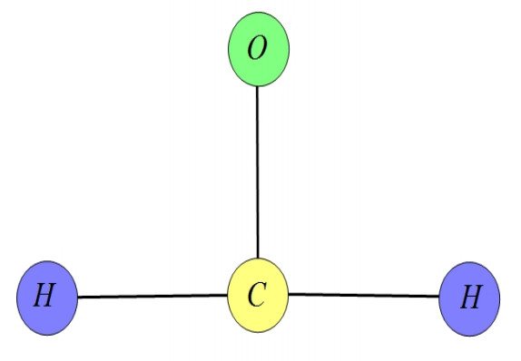
Figure 3 (The structure of formaldehyde) is from reference[22]. Coordinate systems with $ r_{1}, \; r_{2}, $ and $ r_{3} $ are established, respectively, on the formaldehyde graph with 3 edges (Figure 4).
For$ t\in [1, e], $
| $ g1(t,r1(t),HDβ1+r1(t))=1+15(t+3)2(sin(r1(t)+|HD341+r1(t)|1+|HD341+r1(t)|),g2(t,r2(t),HDβ1+r2(t))=1+1(t+2)7(sin(r2(t)+|HD341+r2(t)|1+|HD341+r2(t)|),g3(t,r3(t),HDβ1+r3(t))=1+t1000|arcsin(r3(t))|+t|HD341+r3(t)|1000(1+|HD341+r3(t)|). $ |
For any $ x, \; y, \; x_{1}, \; y_{1} $, it is clear that
| $ g_{1}(t,x,y)-g_{1}(t,x_{1},y_{1})\leq\frac{1}{5(t+3)^{2}}(|x-x_{1}|+|y-y_{1}|), $ |
| $ g_{2}(t,x,y)-g_{2}(t,x_{2},y_{2})\leq\frac{1}{(t+2)^{7}}(|x-x_{2}|+|y-y_{2}|), $ |
| $ g_{3}(t,x,y)-g_{3}(t,x_{3},y_{3})\leq \frac{t}{1000}(|x-x_{3}|+|y-y_{3}|). $ |
So we get
| $ u_{1} = \sup\limits_{t\in[1,e]}|u_{1}(t)| = \frac{1}{5120}, u_{2} = \sup\limits_{t\in[1,e]}|u_{2}(t)| = \frac{1}{2187}, u_{3} = \sup\limits_{t\in[1,e]}|u_{3}(t)| = \frac{e}{1000}, $ |
| $ \chi_{1} = 51.9811, \chi_{2} = 54.7872, \chi_{3} = 58.0208, $ |
and
| $ (\chi_{1}+\chi_{2}+\chi_{3})(u_{1}+u_{2}+u_{3}) = 0.5555 < 1. $ |
Therefore, by Theorem 3.1, system (5.1) has a unique solution on $ [1, e] $.
Meanwhile,
| $ \theta_{1} = 14.1839,\; \; \; \; \theta_{2} = 9.7755, $ |
| $ A = (2.6581e−037.134e−036.1901e−021.832e−031.0351e−026.1901e−021.832e−037.134e−038.9816e−02). $ |
Let
| $ det(\lambda I-A) = (\lambda-0.0964)(\lambda-0.0011)(\lambda-0.0054) = 0, $ |
so we have
| $ \lambda_{1} = 0.0964 < 1, \; \; \; \lambda_{2} = 0.0011 < 1, \; \; \; \lambda_{3} = 0.0054 < 1. $ |
It follows from Theorem 4.6 that system (5.1) is Hyer-Ulams stable, and by Remark 4.4, it will be generalized Hyer-Ulams stable.
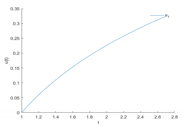
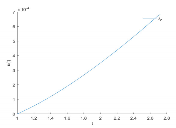
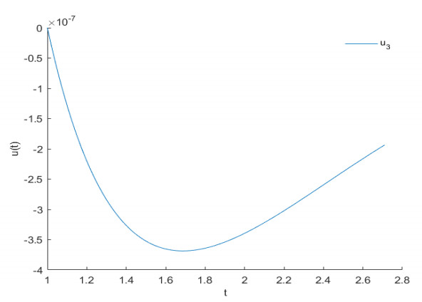
Ultimately, the iterative process curve and approximate solution to the fractional differential system (5.1) are carried out by using the iterative method and numerical simulation. Let $ u_{i, 0} = 0 $, the iteration sequence is as follows:
| $ r1,n+1(t)=−(13)74Γ(74)∫t1(logts)34ϕ3(1+15(t+3)2(sin(r1,n(t))+|HD341+r1,n(t)|1+|HD341+r1,n(t)|))ds−(13)74(12)−1(logt)((13)−1+(12)−1+(23)−1)Γ(74)∫e1(1−logs)34ϕ3(1+1(t+2)7(sin|r2,n(t)|+|HD341+r2,n(t)|1+|HD341+r2,n(t)|))ds−(13)74(12)−1(logt)((13)−1+(12)−1+(23)−1)Γ(74)∫e1(1−logs)34×ϕ3((1+0.001t|arcsin(r3,n(t))|+t|HD341+r3,n(t)|1000+1000|HD341+r3,n(t)|))ds+(12)−1(13)74(logt)((13)−1+(12)−1+(23)−1)Γ(74)∫e1(1−logs)34ϕ3(1+15(t+3)2(sin(r1,n(t))+|HD341+r1,n(t)|1+|HD341+r1,n(t)|))ds+(13)74(23)−1(logt)((13)−1+(12)−1+(23)−1)Γ(74)∫e1(1−logs)34×ϕ3(1+15(t+3)2(sin(r1,n(t))+|HD341+r1,n(t)|1+|HD341+r1,n(t)|))ds+(13)74(13)−1(logt)((13)−1+(12)−1+(23)−1)1Γ(34)∫e1(1−logs)−12ϕ3(1+15(t+3)2×(sin(r1,n(t))+|HD341+r1,n(t)|1+|HD341+r1,n(t)|))ds+(12)52(12)−1(logt)((14)−1+(12)−1+(23)−1)Γ(34)×∫e1(1−logs)−12ϕ3(1+1(t+2)7(sin|r2,n(t)|+|D341+r2,n(t)|1+|D341+r2,n(t)|))ds+(23)74(23)−1(logt)((13)−1+(12)−1+(23)−1)Γ(32)∫e1(1−logs)−12ϕ3(1+0.003t×|arcsin(r3,n(t))|+t|HD341+r3,n(t)|1000+1000|HD341+r3,n(t)|))ds. $ |
The iterative sequence of $ r_{2, n+1} $ and $ r_{3, n+1} $ is similar to $ r_{1, n+1} $. After several iterations, the approximate solution of fractional differential system (5.1) can be obtained by using the numerical simulation. Figure 5 is the approximate graph of the solution of $ \overrightarrow{r_{1}r_{0}} $ after iterations. Figure 6 is the approximate graph of the solution of $ \overrightarrow{r_{2}r_{0}} $ after iterations. Figure 7 is the approximate graph of the solution of $ \overrightarrow{r_{3}r_{0}} $ after iterations.
Using the idea of star graphs, several scholars have studied the solutions of fractional differential equations. They chose to utilize star graphs since their method required a central node connected to nearby vertices through interconnections, but there are no edges between the nodes.
The purpose of this study was to extend the technique's applicability by introducing the concept of a benzoic acid graph, a fundamental molecule in chemistry with the formula $ C_{7}H_{6}O_{2} $. In this manner, we explored a network in which the vertices were either labeled with 0 or 1, and the structure of the chemical molecule benzoic acid was shown to have an effect on this network. To study whether or not there were solutions to the offered boundary value problems within the context of the Caputo fractional derivative with $ p $-Laplacian operators, we used the fixed-point theorems developed by Krasnoselskii. Meanwhile, the Hyers-Ulam stability has been considered. In conclusion, an example was given to illustrate the significance of the findings obtained from this research line.
The following open problems are presented for the consideration of readers interested in this topic: At present, the research prospects of fractional boundary value problems and their numerical solutions on graphs are very broad, which can be extended to other graphs, such as chord bipartite graphs. The follow-up research process, especially the research on chemical graph theory, has a certain practical significance. This is because such research does not need chemical reagents and experimental equipment. In the absence of experimental conditions and reagents, the molecular structure is studied, and the same results are obtained under experimental conditions. Although the differential equation on the benzoic acid graph is studied in this paper, the molecular structure is not studied by the topological index in the research process. It can be tried later to provide a theoretical basis for the study of reverse engineering and provide new ideas for the study of mathematics, chemistry, and other fields.
Yunzhe Zhang: Writing-original draft, formal analysis, investigation; Youhui Su: Supervision, writing-review, editing and project administration; Yongzhen Yu: Resources, editing. All authors have read and approved the final version of the manuscript for publication.
The authors declare they have not used Artificial Intelligence (AI) tools in the creation of this article.
This work is supported by the Xuzhou Science and Technology Plan Project (KC23058) and the Natural Science Research Project of Jiangsu Colleges and Universities (22KJB110026).
The author declares no conflicts of interest.
| [1] | A. Agarwal, S. Das and D. Sen, Power dissipation for systems with junctions of multiple quantum wires, Physical Review B, 81 (2010). |
| [2] | L. Ahlfors, "Complex Analysis," McGraw-Hill, New York, 1966. |
| [3] | F. Ali Mehmeti, "Nonlinear Waves in Networks," Akademie Verlag, Berlin, 1994. |
| [4] |
R. Carlson, Inverse eigenvalue problems on directed graphs, Transactions of the American Mathematical Society, 351 (1999), 4069-4088. doi: 10.1090/S0002-9947-99-02175-3

|
| [5] | R. Carlson, Linear network models related to blood flow, in Quantum Graphs and Their Applications, Contemporary Mathematics, 415 (2006), 65-80. |
| [6] |
C. Cattaneo and L. Fontana, D'Alembert formula on finite one-dimensional networks, J. Math. Anal. Appl., 284 (2003), 403-424. doi: 10.1016/S0022-247X(02)00392-X
|
| [7] |
G. Chen, S. Krantz, D. Russell, C. Wayne, H. West and M. Coleman, Analysis, designs, and behavior of dissipative joints for coupled beams, SIAM Journal on Applied Mathematics., 49 (1989), 1665-1693. doi: 10.1137/0149101
|
| [8] |
S. Cox and E. Zuazua, The rate at which energy decays in a string damped at one end, Indiana Univ. Math. J., 44 (1995), 545-573. doi: 10.1512/iumj.1995.44.2001
|
| [9] |
E. B. Davies, Eigenvalues of an elliptic system, Math. Z., 243 (2003), 719-743. doi: 10.1007/s00209-002-0464-0
|
| [10] | E. B. Davies, P. Exner and J. Lipovsky, Non-Weyl asymptotics for quantum graphs with general coupling conditions, J. Phys. A, 43 (2010). |
| [11] | Y. Fung, "Biomechanics," Springer, New York, 1997. |
| [12] | I. Herstein, "Topics in Algebra," Xerox College Publishing, Waltham, 1964. |
| [13] |
B. Jessen and H. Tornhave, Mean motions and zeros of almost periodic functions, Acta Math., 77 (1945), 137-279. doi: 10.1007/BF02392225
|
| [14] | T. Kato, "Perturbation Theory for Linear Operators," Springer-Verlag, New York, 1995. |
| [15] | V. Kostrykin, J. Potthoff and R. Schrader, Contraction semigroups on metric graphs, in Analysis on Graphs and Its Applications, PSUM, 77 (2008), 423-458. |
| [16] |
T. Kottos and U. Smilansky, Periodic orbit theory and spectral statistics for quantum graphs, Ann. Phys., 274 (1999), 76-124. doi: 10.1006/aphy.1999.5904
|
| [17] |
M. Kramar and E. Sikolya, Spectral properties and asymptotic periodicity of flows in networks, Math. Z., 249 (2005), 139-162. doi: 10.1007/s00209-004-0695-3
|
| [18] |
M. Kramar Fijavz, D. Mugnolo and E. Sikolya, Variational and semigroup methods for waves and diffusions in networks, Appl. Math. Optim., 55 (2007), 219-240. doi: 10.1007/s00245-006-0887-9
|
| [19] | M. Krein and A. Nudelman, Some spectral properties of a nonhomogeneous string with a dissipative boundary condition, J. Operator Theory, 22 (1989), 369-395. |
| [20] | B. Levin, "Distribution of Zeros of Entire Functions," American Mathematical Society, Providence, 1980. |
| [21] | S. Lang, "Algebra," Addison-Wesley, 1984. |
| [22] | G. Lumer, "Equations de Diffusion Generales sur des Reseaux Infinis," Seminar Goulaouic-Schwartz, 1980. |
| [23] | G. Lumer, "Connecting of Local Operators and Evolution Equations on Networks," Lecture Notes in Math., 787, Springer, 1980. |
| [24] | P. Magnusson, G. Alexander, V. Tripathi and A. Weisshaar, "Transmission Lines and Wave Propagation," CRC Press, Boca Raton, 2001. |
| [25] | G. Miano and A. Maffucci, "Transmission Lines and Lumped Circuits," Academic Press, San Diego, 2001. |
| [26] |
L. J. Myers and W. L. Capper, A transmission line model of the human foetal circulatory system, Medical Engineering and Physics, 24 (2002), 285-294. doi: 10.1016/S1350-4533(02)00019-X
|
| [27] | S. Nicaise, Spectre des reseaux topologiques finis, Bulletin des sciences mathematique, 111 (1987), 401-413. |
| [28] |
J. Ottesen, M. Olufsen and J. Larsen, "Applied Mathematical Models in Human Physiology," SIAM, 2004. doi: 10.1137/1.9780898718287
|
| [29] | A. Pazy, "Semigroups of Linear Operators and Applications to Partial Differential Equations," Springer, New York, 1983. |
| [30] |
S. Sherwin, V. Franke, J. Peiro and K. Parker, One-dimensional modeling of a vascular network in space-time variables, Journal of Engineering Mathematics, 47 (2003), 217-250. doi: 10.1023/B:ENGI.0000007979.32871.e2
|
| [31] |
J. von Below, A characteristic equation associated to an eigenvalue problem on C2 networks, Lin. Alg. Appl., 71 (1985), 309-325. doi: 10.1016/0024-3795(85)90258-7
|
| [32] |
L. Zhou and G. Kriegsmann, A simple derivation of microstrip transmission line equations, SIAM J. Appl. Math., 70 (2009), 353-367. doi: 10.1137/080737563
|
| 1. | Okorie Ekwe Agwu, Saad Alatefi, Reda Abdel Azim, Ahmad Alkouh, Applications of artificial intelligence algorithms in artificial lift systems: A critical review, 2024, 97, 09555986, 102613, 10.1016/j.flowmeasinst.2024.102613 | |
| 2. | Okorie Ekwe Agwu, Ahmad Alkouh, Saad Alatefi, Reda Abdel Azim, Razaq Ferhadi, Utilization of machine learning for the estimation of production rates in wells operated by electrical submersible pumps, 2024, 14, 2190-0558, 1205, 10.1007/s13202-024-01761-3 | |
| 3. | Onyebuchi Ivan Nwanwe, Nkemakolam Chinedu Izuwa, Nnaemeka Princewill Ohia, Anthony Kerunwa, Nnaemeka Uwaezuoke, Determining optimal controls placed on injection/production wells during waterflooding in heterogeneous oil reservoirs using artificial neural network models and multi-objective genetic algorithm, 2024, 1420-0597, 10.1007/s10596-024-10300-2 | |
| 4. | Daniel Chuquin-Vasco, Dennise Chicaiza-Sagal, Cristina Calderón-Tapia, Nelson Chuquin-Vasco, Juan Chuquin-Vasco, Lidia Castro-Cepeda, Forecasting mixture composition in the extractive distillation of n-hexane and ethyl acetate with n-methyl-2-pyrrolidone through ANN for a preliminary energy assessment, 2024, 12, 2333-8334, 439, 10.3934/energy.2024020 | |
| 5. | Mariea Marcu, Approximation methods used to build the gas-lift performance curve based on reduced datasets: a comprehensive statistical comparison, 2024, 1091-6466, 1, 10.1080/10916466.2024.2404625 | |
| 6. | Sungil Kim, Tea-Woo Kim, Suryeom Jo, Artificial intelligence in geoenergy: bridging petroleum engineering and future-oriented applications, 2025, 15, 2190-0558, 10.1007/s13202-025-01939-3 | |
| 7. | James O. Arukhe, Ammal F. Anazi, 2025, Predicting Gas Lift Equipment Failure with Deep Learning Techniques, 10.4043/35605-MS |
Robert Carlson. Spectral theory for nonconservative transmission line networks[J]. Networks and Heterogeneous Media, 2011, 6(2): 257-277. doi: 10.3934/nhm.2011.6.257

 DownLoad:
