Ultrasound carotid plaque segmentation via image reconstruction-based self-supervised learning with limited training labels

Ran Zhou; Yanghan Ou; Xiaoyue Fang; M. Reza Azarpazhooh; Haitao Gan; Zhiwei Ye; J. David Spence; Xiangyang Xu; Aaron Fenster; Ran Zhou; Yanghan Ou; Xiaoyue Fang; M. Reza Azarpazhooh; Haitao Gan; Zhiwei Ye; J. David Spence; Xiangyang Xu; Aaron Fenster

doi:10.3934/mbe.2023074

Mathematical Biosciences and Engineering

2023, Volume 20, Issue 2: 1617-1636. doi: 10.3934/mbe.2023074

Previous Article Next Article

Research article Special Issues

Ultrasound carotid plaque segmentation via image reconstruction-based self-supervised learning with limited training labels

1.
School of Computer Science, Hubei University of Technology, Wuhan, China
2.
Robarts Research Institute, Western University, London, Canada
3.
Liyuan Hospital, Tongji Medical College, Huazhong University of Science and Technology, Wuhan, China
Academic editor: Biswajeet Pradhan

Received: 09 August 2022 Revised: 09 October 2022 Accepted: 13 October 2022 Published: 03 November 2022

Carotid total plaque area (TPA) is an important contributing measurement to the evaluation of stroke risk. Deep learning provides an efficient method for ultrasound carotid plaque segmentation and TPA quantification. However, high performance of deep learning requires datasets with many labeled images for training, which is very labor-intensive. Thus, we propose an image reconstruction-based self-supervised learning algorithm (IR-SSL) for carotid plaque segmentation when few labeled images are available. IR-SSL consists of pre-trained and downstream segmentation tasks. The pre-trained task learns region-wise representations with local consistency by reconstructing plaque images from randomly partitioned and disordered images. The pre-trained model is then transferred to the segmentation network as the initial parameters in the downstream task. IR-SSL was implemented with two networks, UNet++ and U-Net, and evaluated on two independent datasets of 510 carotid ultrasound images from 144 subjects at SPARC (London, Canada) and 638 images from 479 subjects at Zhongnan hospital (Wuhan, China). Compared to the baseline networks, IR-SSL improved the segmentation performance when trained on few labeled images (n = 10, 30, 50 and 100 subjects). For 44 SPARC subjects, IR-SSL yielded Dice-similarity-coefficients (DSC) of 80.14–88.84%, and algorithm TPAs were strongly correlated ($ r = 0.962 - 0.993 $, $ p $ < 0.001) with manual results. The models trained on the SPARC images but applied to the Zhongnan dataset without retraining achieved DSCs of 80.61–88.18% and strong correlation with manual segmentation ($ r = 0.852 - 0.978 $, $ p $ < 0.001). These results suggest that IR-SSL could improve deep learning when trained on small labeled datasets, making it useful for monitoring carotid plaque progression/regression in clinical use and trials.
- carotid plaque,
- ultrasound image segmentation,
- self-supervised learning,
- convolutional neural network
Citation: Ran Zhou, Yanghan Ou, Xiaoyue Fang, M. Reza Azarpazhooh, Haitao Gan, Zhiwei Ye, J. David Spence, Xiangyang Xu, Aaron Fenster. Ultrasound carotid plaque segmentation via image reconstruction-based self-supervised learning with limited training labels[J]. Mathematical Biosciences and Engineering, 2023, 20(2): 1617-1636. doi: 10.3934/mbe.2023074

Related Papers:

Abstract

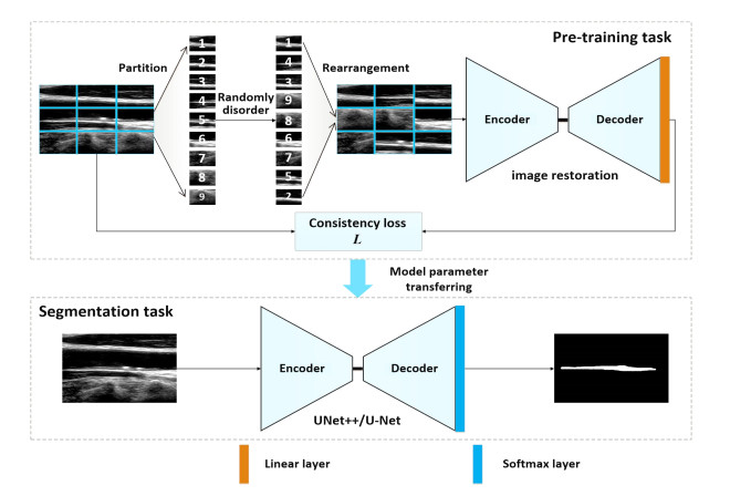
Carotid total plaque area (TPA) is an important contributing measurement to the evaluation of stroke risk. Deep learning provides an efficient method for ultrasound carotid plaque segmentation and TPA quantification. However, high performance of deep learning requires datasets with many labeled images for training, which is very labor-intensive. Thus, we propose an image reconstruction-based self-supervised learning algorithm (IR-SSL) for carotid plaque segmentation when few labeled images are available. IR-SSL consists of pre-trained and downstream segmentation tasks. The pre-trained task learns region-wise representations with local consistency by reconstructing plaque images from randomly partitioned and disordered images. The pre-trained model is then transferred to the segmentation network as the initial parameters in the downstream task. IR-SSL was implemented with two networks, UNet++ and U-Net, and evaluated on two independent datasets of 510 carotid ultrasound images from 144 subjects at SPARC (London, Canada) and 638 images from 479 subjects at Zhongnan hospital (Wuhan, China). Compared to the baseline networks, IR-SSL improved the segmentation performance when trained on few labeled images (n = 10, 30, 50 and 100 subjects). For 44 SPARC subjects, IR-SSL yielded Dice-similarity-coefficients (DSC) of 80.14–88.84%, and algorithm TPAs were strongly correlated ($ r = 0.962 - 0.993 $, $ p $ < 0.001) with manual results. The models trained on the SPARC images but applied to the Zhongnan dataset without retraining achieved DSCs of 80.61–88.18% and strong correlation with manual segmentation ($ r = 0.852 - 0.978 $, $ p $ < 0.001). These results suggest that IR-SSL could improve deep learning when trained on small labeled datasets, making it useful for monitoring carotid plaque progression/regression in clinical use and trials.

References

[1]	T. Vos, S. S. Lim, C. Abbafati, K. M. Abbas, M. Abbasi, M. Abbasifard, et al., Global burden of 369 diseases and injuries in 204 countries and territories, 1990–2019: A systematic analysis for the global burden of disease study 2019, Lancet, 369 (2020), 1204–1222. https://doi.org/10.1016/S0140-6736(20)30925-9 doi: 10.1016/S0140-6736(20)30925-9
[2]	J. D. Spence, Technology insight: Ultrasound measurement of carotid plaque-patient management, genetic research, and therapy evaluation, Nat. Clin. Pract. Neurol., 2 (2006), 611–619. https://doi.org/10.1038/ncpneuro0324 doi: 10.1038/ncpneuro0324
[3]	M. L. Bots, A. W. Hoes, P. J. Koudstaal, A. Hofman, D. E. Grobbee, Common carotid intima-media thickness and risk of stroke and myocardial infarction: The rotterdam study, Circulation, 96 (1997), 1432–143. https://doi.org/10.1161/01.cir.96.5.1432 doi: 10.1161/01.cir.96.5.1432
[4]	J. D. Spence, Carotid ultrasound phenotypes are biologically distinct, Arterioscler., Thromb., Vasc. Biol., 35 (2015), 1910–1913. https://doi.org/10.1161/ATVBAHA.115.306209 doi: 10.1161/ATVBAHA.115.306209
[5]	A. V. Finn, F. D. Kolodgie, R. Virmani, Correlation between carotid intimal/medial thickness and atherosclerosis: A point of view from pathology, Arterioscler., Thromb., Vasc. Biol., 30 (2010), 177–181. https://doi.org/10.1161/ATVBAHA.108.173609 doi: 10.1161/ATVBAHA.108.173609
[6]	R. L. Pollex, R. A. Hegele, Genetic determinants of carotid ultrasound traits, Curr. Atheroscler. Rep., 8 (2006), 206–215. https://doi.org/10.1007/s11883-006-0075-z doi: 10.1007/s11883-006-0075-z
[7]	E. B. Mathiesen, S. H. Johnsen, T. Wilsgaard, K. H. Bønaa, M. L. Løchen, I. Njølstad, Carotid plaque area and intima-media thickness in prediction of first-ever ischemic stroke: A 10-year follow-up of 6584 men and women: the tromsø study, Stroke, 42 (2011), 972–978. https://doi.org/10.1161/strokeaha.110.589754 doi: 10.1161/strokeaha.110.589754
[8]	C. Loizou, S. Petroudi, M. Pantziaris, A. Nicolaides, C. Pattichis, An integrated system for the segmentation of atherosclerotic carotid plaque ultrasound video, IEEE Trans. Ultrason. Ferroelectr. Freq. Control, 61 (2014), 86–101. https://doi.org/10.1109/tuffc.2014.6689778 doi: 10.1109/tuffc.2014.6689778
[9]	J. Cheng, H. Li, F. Xiao, A. Fenster, X. Zhang, X. He, et al., Fully automatic plaque segmentation in 3-D carotid ultrasound images, Ultrasound Med. Biol., 39 (2013), 2431–2446. https://doi.org/10.1016/j.ultrasmedbio.2013.07.007 doi: 10.1016/j.ultrasmedbio.2013.07.007
[10]	F. Destrempes, J. Meunier, M. F. Giroux, G. Soulez, G. Cloutier, Segmentation of plaques in sequences of ultrasonic b-mode images of carotid arteries based on motion estimation and a bayesian model, IEEE Trans. Biomed. Eng., 58 (2011), 2202–2211. https://doi.org/10.1109/tbme.2011.2127476 doi: 10.1109/tbme.2011.2127476
[11]	S. Delsanto, F. Molinari, P. Giustetto, W. Liboni, S. Badalamenti, J. S. Suri, Characterization of a completely user-independent algorithm for carotid artery segmentation in 2-D ultrasound images, IEEE Trans. Instrum. Meas., 56 (2007), 1265–1274. https://doi.org/10.1109/TIM.2007.900433 doi: 10.1109/TIM.2007.900433
[12]	R. M. Menchón-Lara, M. C. Bastida-Jumilla, J. Morales-Sánchez, J. L. Sancho-Gómez, Automatic detection of the intima-media thickness in ultrasound images of the common carotid artery using neural networks, Med. Biol. Eng. Comput., 52 (2014), 169–181. https://doi.org/10.1007/s11517-013-1128-4 doi: 10.1007/s11517-013-1128-4
[13]	C. Azzopardi, Y. A. Hicks, K. P. Camilleri, Automatic carotid ultrasound segmentation using deep convolutional neural networks and phase congruency maps, in 2017 IEEE 14th International Symposium on Biomedical Imaging (ISBI 2017), (2017), 624–628. https://doi.org/10.1109/ISBI.2017.7950598
[14]	S. Savaş, N. Topaloğlu, O. Kazcı, P. N. Koşar, Classification of carotid artery intima media thickness ultrasound images with deep learning, J. Med. Syst., 43 (2019), 273. https://doi.org/10.1007/s10916-019-1406-2 doi: 10.1007/s10916-019-1406-2
[15]	C. Qian, E. Su, X. Yang, Segmentation of the common carotid intima-media complex in ultrasound images using 2-D continuous max-flow and stacked sparse auto-encoder, Ultrasound Med. Biol., 46 (2020), 3104–3124. https://doi.org/10.1016/j.ultrasmedbio.2020.07.021 doi: 10.1016/j.ultrasmedbio.2020.07.021
[16]	M. Jiang, Y. Zhao, B. Chiu, Segmentation of common and internal carotid arteries from 3D ultrasound images based on adaptive triple loss, Med. Phys., 48 (2021), 5096–5114. https://doi.org/10.1002/mp.15127 doi: 10.1002/mp.15127
[17]	R. Zhou, A. Fenster, Y. Xia, J. D. Spence, M. Ding, Deep learning-based carotid media-adventitia and lumen-intima boundary segmentation from three-dimensional ultrasound images, Med. Phys., 46 (2019), 3180–3193. https://doi.org/10.1002/mp.13581 doi: 10.1002/mp.13581
[18]	R. Zhou, F. Guo, M. R. Azarpazhooh, J. D. Spence, E. Ukwatta, M. Ding, A. Fenster, A voxel-based fully convolution network and continuous max-flow for carotid vessel-wall-volume segmentation from 3D ultrasound images, IEEE Trans. Med. Imaging, 39 (2020), 2844–2855. https://doi.org/10.1109/tmi.2020.2975231 doi: 10.1109/tmi.2020.2975231
[19]	R. Zhou, F. Guo, M. R. Azarpazhooh, S. Hashemi, X. Cheng, J. D. Spence, et al., Deep learning-based measurement of total plaque area in b-mode ultrasound images, IEEE J Biomed. Health Inform., 25 (2021), 2967–2977. https://doi.org/10.1109/jbhi.2021.3060163 doi: 10.1109/jbhi.2021.3060163
[20]	C. Doersch, A. Zisserman, Multi-task self-supervised visual learning, in 2017 IEEE International Conference on Computer Vision(ICCV), (2017), 2070–2079. https://doi.org/10.1109/ICCV.2017.226
[21]	Z. Ren, Y. J. Lee, Cross-domain self-supervised multi-task feature learning using synthetic imagery, in 2018 IEEE/CVF Conference on Computer Vision and Pattern Recognition, (2018). http://dx.doi.org/10.1109/CVPR.2018.00086
[22]	X. Zheng, Y. Wang, G. Wang, J. Liu, Fast and robust segmentation of white blood cell images by self-supervised learning, Micron, 107 (2018), 55–71. https://doi.org/10.1016/j.micron.2018.01.010 doi: 10.1016/j.micron.2018.01.010
[23]	L. Chen, P. Bentley, K. Mori, K. Misawa, M. Fujiwara, D. Rueckert, Self-supervised learning for medical image analysis using image context restoration, Med. Image Anal., 58 (2019), 101539. https://doi.org/10.1016/j.media.2019.101539 doi: 10.1016/j.media.2019.101539
[24]	X. Zhuang, Y. Li, Y. Hu, K. Ma, Y. Yang, Y. Zheng, Self-supervised feature learning for 3D medical images by playing a rubik's cube, in International Conference on Medical Image Computing and Computer-Assisted Intervention, (2019), 420–428. https://doi.org/10.1007/978-3-030-32251-9_46
[25]	Q. Lu, Y. Li, C. Ye, White matter tract segmentation with self-supervised learning, in International Conference on Medical Image Computing and Computer-Assisted Intervention, (2020), 270–279. https://doi.org/10.1007/978-3-030-59728-3_27
[26]	J. D. Spence, M. Eliasziw, M. Dicicco, D. G. Hackam, R. Galil, T. Lohmann, Carotid plaque area: A tool for targeting and evaluating vascular preventive therapy, Stroke, 33 (2002), 2916–2922. https://doi.org/10.1161/01.str.0000042207.16156.b9 doi: 10.1161/01.str.0000042207.16156.b9
[27]	S. H. Johnsen, E. B. Mathiesen, O. Joakimsen, E. Stensland, T. Wilsgaard, M.L. Løchen, et al., Carotid atherosclerosis is a stronger predictor of myocardial infarction in women than in men: A 6-year follow-up study of 6226 persons: the tromsø study, Stroke, 38 (2007), 2873–2880. https://doi.org/10.1161/strokeaha.107.487264 doi: 10.1161/strokeaha.107.487264
[28]	M. Noroozi, P. Favaro, Unsupervised learning of visual representations by solving jigsaw puzzles, in European Conference on Computer Vision, (2016), 69–84. https://doi.org/10.1007/978-3-319-46466-4_5
[29]	O. Ronneberger, P. Fischer, T. Brox, U-net: Convolutional networks for biomedical image segmentation, in International Conference on Medical Image Computing and Computer-Assisted Intervention, (2015), 234–241. https://doi.org/10.1007/978-3-319-24574-4_28
[30]	Z. Zhou, M. M. R. Siddiquee, N. Tajbakhsh, J. Liang, Unet++: Redesigning skip connections to exploit multiscale features in image segmentation, IEEE Trans. Med. Imaging, 39 (2020), 1856–1867. https://doi.org/10.1109/tmi.2019.2959609 doi: 10.1109/tmi.2019.2959609
[31]	R. Zhou, M. R. Azarpazhooh, J. D. Spence, S. Hashemi, W. Ma, X. Cheng, et al., Deep learning-based carotid plaque segmentation from b-mode ultrasound images, Ultrasound in Medicine & Biology, 47 (2021), 2723–2733. https://doi.org/10.1016/j.ultrasmedbio.2021.05.023 doi: 10.1016/j.ultrasmedbio.2021.05.023
[32]	K. He, X. Zhang, S. Ren, J. Sun, Deep residual learning for image recognition, Proceedings of the IEEE conference on computer vision and pattern recognition, 2016,770–778. https://doi.org/10.1109/CVPR.2016.90
[33]	T. Heimann, B. V. Ginneken, M. A Styner, Y. Arzhaeva, V. Aurich, C. Bauer, et al., Comparison and evaluation of methods for liver segmentation from CT datasets, IEEE transactions on medical imaging, 28 (2009), 1251–1265. https://doi.org/10.1109/TMI.2009.2013851 doi: 10.1109/TMI.2009.2013851

Reader Comments

Your name:*

Email:*
© 2023 the Author(s), licensee AIMS Press. This is an open access article distributed under the terms of the Creative Commons Attribution License (http://creativecommons.org/licenses/by/4.0)