Bio-inspired negotiation approach for smart-grid colocation datacenter operation

Santiago Iturriaga; Jonathan Muraña; Sergio Nesmachnow; Santiago Iturriaga; Jonathan Muraña; Sergio Nesmachnow

doi:10.3934/mbe.2022111

Mathematical Biosciences and Engineering

2022, Volume 19, Issue 3: 2403-2423. doi: 10.3934/mbe.2022111

Previous Article Next Article

Research article Special Issues

Bio-inspired negotiation approach for smart-grid colocation datacenter operation

Department of Computer Science, Universidad de la República, Julio Herrera y Reissig 565, Montevideo, Uruguay

Academic Editor: Guadalupe Ortiz Bellot

Received: 28 September 2021 Revised: 13 December 2021 Accepted: 19 December 2021 Published: 05 January 2022

Demand response programs allow consumers to participate in the operation of a smart electric grid by reducing or shifting their energy consumption, helping to match energy consumption with power supply. This article presents a bio-inspired approach for addressing the problem of colocation datacenters participating in demand response programs in a smart grid. The proposed approach allows the datacenter to negotiate with its tenants by offering monetary rewards in order to meet a demand response event on short notice. The objective of the underlying optimization problem is twofold. The goal of the datacenter is to minimize its offered rewards while the goal of the tenants is to maximize their profit. A two-level hierarchy is proposed for modeling the problem. The upper-level hierarchy models the datacenter planning problem, and the lower-level hierarchy models the task scheduling problem of the tenants. To address these problems, two bio-inspired algorithms are designed and compared for the datacenter planning problem, and an efficient greedy scheduling heuristic is proposed for task scheduling problem of the tenants. Results show the proposed approach reports average improvements between $ 72.9\% $ and $ 82.2\% $ when compared to the business as usual approach.
- smart grid,
- demand response,
- colocation datacenter,
- evolutionary negotiation
Citation: Santiago Iturriaga, Jonathan Muraña, Sergio Nesmachnow. Bio-inspired negotiation approach for smart-grid colocation datacenter operation[J]. Mathematical Biosciences and Engineering, 2022, 19(3): 2403-2423. doi: 10.3934/mbe.2022111

Related Papers:

Abstract

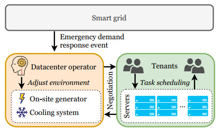
Demand response programs allow consumers to participate in the operation of a smart electric grid by reducing or shifting their energy consumption, helping to match energy consumption with power supply. This article presents a bio-inspired approach for addressing the problem of colocation datacenters participating in demand response programs in a smart grid. The proposed approach allows the datacenter to negotiate with its tenants by offering monetary rewards in order to meet a demand response event on short notice. The objective of the underlying optimization problem is twofold. The goal of the datacenter is to minimize its offered rewards while the goal of the tenants is to maximize their profit. A two-level hierarchy is proposed for modeling the problem. The upper-level hierarchy models the datacenter planning problem, and the lower-level hierarchy models the task scheduling problem of the tenants. To address these problems, two bio-inspired algorithms are designed and compared for the datacenter planning problem, and an efficient greedy scheduling heuristic is proposed for task scheduling problem of the tenants. Results show the proposed approach reports average improvements between $ 72.9\% $ and $ 82.2\% $ when compared to the business as usual approach.

References

[1]	J. Momoh, Smart grid: Fundamentals of design and analysis, Wiley IEEE Press, 2012.
[2]	H. Fraser, The importance of an active demand side in the electricity industry, Electr. J., 14 (2001), 52–73. https://doi.org/10.1016/S1040-6190(01)00249-4 doi: 10.1016/S1040-6190(01)00249-4
[3]	M. Chen, C. Gao, M. Song, S. Chen, D. Li, Q. Liu, Internet data centers participating in demand response: A comprehensive review, Renew. Sustain. Energy Rev., 117 (2020), 1–15. https://doi.org/10.1016/j.rser.2019.109466 doi: 10.1016/j.rser.2019.109466
[4]	J. Muraña, S. Nesmachnow, S. Iturriaga, S. M. de Oca, G. Belcredi, P. Monzón, et al., Two level demand response planning for retail multi-tenant datacenters, in 18th International Conference on High Performance Computing and Simulation, (2021), 1–8.
[5]	F. L. Meng, X. J. Zeng, A Stackelberg game-theoretic approach to optimal real-time pricing for the smart grid, Soft Comput., 17 (2013), 2365–2380. https://doi.org/10.1007/s00500-013-1092-9 doi: 10.1007/s00500-013-1092-9
[6]	K. Alshehri, J. Liu, X. Chen, T. Basar, A Stackelberg game for multi-period demand response management in the smart grid, in 54th IEEE Conference on Decision and Control, (2015), 5889–5894. https://doi.org/10.1109/CDC.2015.7403145
[7]	M. Yu, S. Hong, Supply-demand balancing for power management in smart grid: A Stackelberg game approach, Appl. Energy, 164 (2016), 702–710. https://doi.org/10.1016/j.apenergy.2015.12.039 doi: 10.1016/j.apenergy.2015.12.039
[8]	Y. Dai, Y. Gao, H. Gao, H. Zhu, Real-time pricing scheme based on Stackelberg game in smart grid with multiple power retailers, Neurocomputing, 260 (2017), 149–156. http://doi.org/10.1016/j.neucom.2017.04.027 doi: 10.1016/j.neucom.2017.04.027
[9]	Y. Wang, X. Lin, M. Pedram, A Stackelberg game-based optimization framework of the smart grid with distributed PV power generations and data centers, IEEE Trans. Energy Conver., 29 (2014), 978–987. https://doi.org/10.1109/TEC.2014.2363048 doi: 10.1109/TEC.2014.2363048
[10]	N. Chen, X. Ren, S. Ren, A. Wierman, Greening multi-tenant data center demand response, Perform. Eval., 91 (2015), 229–254. https://doi.org/10.1016/j.peva.2015.06.014 doi: 10.1016/j.peva.2015.06.014
[11]	M. N. H. Nguyen, D. Kim, N. H. Tran, C. S. Hong, Multi-stage Stackelberg game approach for colocation datacenter demand response, in 19th Asia-Pacific Network Operations and Management Symposium, (2017), 139–144. https://doi.org/10.1109/APNOMS.2017.8094193
[12]	C. Chi, F. Zhang, K. Ji, A. Marahatta, Z. Liu, Improving energy efficiency in colocation data centers for demand response, Sustain. Comput. Infor. Syst., 29 (2021), 100476. https://doi.org/10.1016/j.suscom.2020.100476 doi: 10.1016/j.suscom.2020.100476
[13]	L. Zhang, S. Ren, C. Wu, Z. Li, A truthful incentive mechanism for emergency demand response in colocation data centers, in IEEE Conference on Computer Communications, (2015), 2632–2640. https://doi.org/10.1109/INFOCOM.2015.7218654
[14]	J. Chen, D. Ye, S. Ji, Q. He, Y. Xiang, Z. Liu, A truthful FPTAS mechanism for emergency demand response in colocation data centers, in IEEE Conference on Computer Communications, (2019), 2557–2565. https://doi.org/10.1109/INFOCOM.2019.8737468
[15]	B. Celik, G. Rostirolla, S. Caux, P. Renaud-Goud, P. Stolf, Analysis of demand response for datacenter energy management using GA and time-of-use prices, in IEEE PES Innovative Smart Grid Technologies Europe, (2019), 1–5. https://doi.org/10.1109/ISGTEurope.2019.8905618
[16]	J. Muraña, S. Nesmachnow, S. Iturriaga, S. M. de Oca, G. Belcredi, P. Monzón, et al., Negotiation approach for the participation of datacenters and supercomputing facilities in smart electricity markets, Program. Comput. Software, 46 (2020), 636–651. https://doi.org/10.1134/S0361768820080150 doi: 10.1134/S0361768820080150
[17]	J. Muraña, S. Nesmachnow, Simulation and evaluation of multicriteria planning heuristics for demand response in datacenters, Simulation, (2021), 1–18. https://doi.org/10.1177/00375497211020083
[18]	J. Muraña, S. Nesmachnow, F. Armenta, A. Tchernykh, Characterization, modeling and scheduling of power consumption of scientific computing applications in multicores, Cluster Comput., 22 (2019), 839–859. https://doi.org/10.1007/s10586-018-2882-8 doi: 10.1007/s10586-018-2882-8
[19]	N. H. Tran, C. Pham, S. Ren, Z. Han, C. S. Hong, Coordinated power reduction in multi-tenant colocation datacenter: An emergency demand response study, in IEEE International Conference on Communications, (2016), 1–6. https://doi.org/10.1109/ICC.2016.7511560
[20]	C. Cowden, Game theory, evolutionary stable strategies and the evolution of biological interactions, Nat. Educ. Knowl., 3 (2012), 1–6.
[21]	H. Stackelberg, The theory of the market economy, Oxford University Press, 1952.
[22]	D. E. Goldberg, Genetic algorithms in search, optimization, and machine learning, Addison-Wesley, 1989.
[23]	K. Deb, R. B. Agrawal, Simulated binary crossover for continuous search space, Complex syst., 9 (1995), 115–148.
[24]	K. Deb, S. Tiwari, Omni-optimizer: A generic evolutionary algorithm for single and multi-objective optimization, Eur. J. Oper. Res., 185 (2008), 1062–1087. https://doi.org/10.1016/j.ejor.2006.06.042 doi: 10.1016/j.ejor.2006.06.042
[25]	D. E. Goldberg, K. Deb, A comparative analysis of selection schemes used in genetic algorithms, Found. Genet. Algorithms, 1 (1991), 69–93, https://doi.org/10.1016/B978-0-08-050684-5.50008-2 doi: 10.1016/B978-0-08-050684-5.50008-2
[26]	J. Kennedy, R. Eberhart, Particle swarm optimization, in Proceedings of International Conference on Neural Networks, (1995), 1942–1948. https://doi.org/10.1109/ICNN.1995.488968
[27]	G. Beni, J. Wang, Swarm intelligence in cellular robotic systems, in Robots and Biological Systems: Towards a New Bionics?, (1993), 703–712. https://doi.org/10.1007/978-3-642-58069-7_38
[28]	M. Zambrano-Bigiarini, M. Clerc, R. Rojas, Standard particle swarm optimisation 2011 at CEC-2013: A baseline for future PSO improvements, in IEEE Congress on Evolutionary Computation, (2013), 2337–2344. https://doi.org/10.1109/CEC.2013.6557848
[29]	M. Clerc, Particle swarm optimization, John Wiley and Sons, 2010.
[30]	A. Gandhi, M. Harchol-Balter, R. Raghunatha, M. A. Kozuch, Autoscale: Dynamic, robust capacity management for multi-tier data centers, ACM Trans. Comp. Sys., 30 (2012), 1–26. https://doi.org/10.1145/2382553.2382556 doi: 10.1145/2382553.2382556
[31]	M. Lin, A. Wierman, L. L. Andrew, E. Thereska, Dynamic right-sizing for power-proportional data centers, IEEE ACM Trans. Netw., 21 (2012), 1378–1391. https://doi.org/10.1109/INFCOM.2011.5934885 doi: 10.1109/INFCOM.2011.5934885
[32]	D. G. Feitelson, D. Tsafrir, D. Krakov, Experience with using the parallel workloads archive, J. Parallel Distrib. Comput., 74 (2014), 2967–2982. https://doi.org/10.1016/j.jpdc.2014.06.013 doi: 10.1016/j.jpdc.2014.06.013
[33]	L. A. Barroso, U. Hölzle, P. Ranganathan, The datacenter as a computer: Designing warehouse-scale machines, Morgan and Claypool Publishers LLC, 2018.
[34]	V. Oladokun, O. Asemota, Unit cost of electricity in Nigeria: A cost model for captive diesel powered generating system, Renew. Sustain. Energy Rev., 52 (2015), 35–40. https://doi.org/10.1016/j.rser.2015.07.028 doi: 10.1016/j.rser.2015.07.028
[35]	J. Durillo, A. Nebro, jMetal: A Java framework for multi-objective optimization, Adv. Eng. Software, 42 (2011), 760–771. https://doi.org/10.1016/j.advengsoft.2011.05.014 doi: 10.1016/j.advengsoft.2011.05.014
[36]	A. Eiben, R. Hinterding, Z. Michalewicz, Parameter control in evolutionary algorithms, IEEE Trans. Evol. Comput., 3 (1999), 124–141. https://doi.org/10.1109/4235.771166 doi: 10.1109/4235.771166
[37]	A. E. Eiben, S. K. Smit, Evolutionary Algorithm Parameters and Methods to Tune Them, Springer, (2012), 15–36.
[38]	X. S. Yang, Flower pollination algorithm for global optimization, in Unconventional Computation and Natural Computation, (2012), 240–249. https://doi.org/10.1007/978-3-642-32894-7_27
[39]	A. A. Heidari, S. Mirjalili, H. Faris, I. Aljarah, M. Mafarja, H. Chen, Harris hawks optimization: Algorithm and applications, Future Gener. Comput. Syst., 97 (2019), 849–872. https://doi.org/10.1016/j.future.2019.02.028 doi: 10.1016/j.future.2019.02.028

Reader Comments

Your name:*

Email:*
© 2022 the Author(s), licensee AIMS Press. This is an open access article distributed under the terms of the Creative Commons Attribution License (http://creativecommons.org/licenses/by/4.0)