Automatic liver segmentation is a prerequisite for hepatoma treatment; however, the low accuracy and stability hinder its clinical application. To alleviate this limitation, we deeply mine the context information of different scales and combine it with deep supervision to improve the accuracy of liver segmentation in this paper.
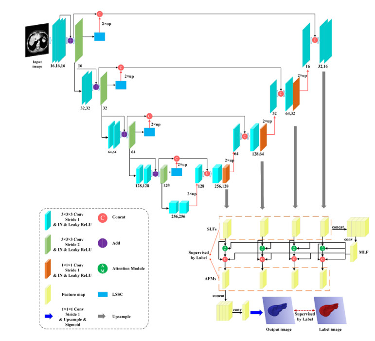
We proposed a new network called MAD-UNet for automatic liver segmentation from CT. It is grounded in the 3D UNet and leverages multi-scale attention and deep supervision mechanisms. In the encoder, the downsampling pooling in 3D UNet is replaced by convolution to alleviate the loss of feature information. Meanwhile, the residual module is introduced to avoid gradient vanishment. Besides, we use the long-short skip connections (LSSC) to replace the ordinary skip connections to preserve more edge detail. In the decoder, the features of different scales are aggregated, and the attention module is employed to capture the spatial context information. Moreover, we utilized the deep supervision mechanism to improve the learning ability on deep and shallow information.
We evaluated the proposed method on three public datasets, including, LiTS17, SLiver07, and 3DIRCADb, and obtained Dice scores of 0.9727, 0.9752, and 0.9691 for liver segmentation, respectively, which outperform the other state-of-the-art (SOTA) methods.
Both qualitative and quantitative experimental results demonstrate that the proposed method can make full use of the feature information of different stages while enhancing spatial data's learning ability, thereby achieving high liver segmentation accuracy. Thus, it proved to be a promising tool for automatic liver segmentation in clinical assistance.
Citation: Jinke Wang, Xiangyang Zhang, Liang Guo, Changfa Shi, Shinichi Tamura. Multi-scale attention and deep supervision-based 3D UNet for automatic liver segmentation from CT[J]. Mathematical Biosciences and Engineering, 2023, 20(1): 1297-1316. doi: 10.3934/mbe.2023059
Automatic liver segmentation is a prerequisite for hepatoma treatment; however, the low accuracy and stability hinder its clinical application. To alleviate this limitation, we deeply mine the context information of different scales and combine it with deep supervision to improve the accuracy of liver segmentation in this paper.
We proposed a new network called MAD-UNet for automatic liver segmentation from CT. It is grounded in the 3D UNet and leverages multi-scale attention and deep supervision mechanisms. In the encoder, the downsampling pooling in 3D UNet is replaced by convolution to alleviate the loss of feature information. Meanwhile, the residual module is introduced to avoid gradient vanishment. Besides, we use the long-short skip connections (LSSC) to replace the ordinary skip connections to preserve more edge detail. In the decoder, the features of different scales are aggregated, and the attention module is employed to capture the spatial context information. Moreover, we utilized the deep supervision mechanism to improve the learning ability on deep and shallow information.
We evaluated the proposed method on three public datasets, including, LiTS17, SLiver07, and 3DIRCADb, and obtained Dice scores of 0.9727, 0.9752, and 0.9691 for liver segmentation, respectively, which outperform the other state-of-the-art (SOTA) methods.
Both qualitative and quantitative experimental results demonstrate that the proposed method can make full use of the feature information of different stages while enhancing spatial data's learning ability, thereby achieving high liver segmentation accuracy. Thus, it proved to be a promising tool for automatic liver segmentation in clinical assistance.

| [1] | H. A. Nugroho, D. Ihtatho, H. Nugroho, Contrast enhancement for liver tumor identification, in MICCAI Workshop, 41 (2008), 201. https://doi.org/10.54294/1uhwld |
| [2] |
D. Wong, J. Liu, Y. Fengshou, Q. Tian, W. Xiong, J. Zhou, et al., A semi-automated method for liver tumor segmentation based on 2D region growing with knowledge-based constraints, MICCAI Workshop, 41 (2008), 159. https://doi.org/10.54294/25etax doi: 10.54294/25etax

|
| [3] |
Y. Yuan, Y. Chen, C. Dong, H. Yu, Z. Zhu, Hybrid method combining superpixel, random walk and active contour model for fast and accurate liver segmentation, Comput. Med. Imaging Graphics, 70 (2018), 119–134. https://doi.org/10.1016/j.compmedimag.2018.08.012 doi: 10.1016/j.compmedimag.2018.08.012
|
| [4] |
J. Wang, Y. Cheng, C. Guo, Y. Wang, S. Tamura, Shape-intensity prior level set combining probabilistic atlas and probability map constrains for automatic liver segmentation from abdominal CT images, Int. J. Comput. Assisted Radiol. Surg., 11 (2016), 817–826. https://doi.org/10.1007/s11548-015-1332-9 doi: 10.1007/s11548-015-1332-9
|
| [5] |
C. Shi, M. Xian, X, Zhou, H. Wang, H. Cheng, Multi-slice low-rank tensor decomposition based multi-atlas segmentation: Application to automatic pathological liver CT segmentation, Med. Image Anal., 73 (2021), 102152. https://doi.org/10.1016/j.media.2021.102152 doi: 10.1016/j.media.2021.102152
|
| [6] |
Z. Yan, S. Zhang, C. Tan, H. Qin, B. Belaroussi, H. J. Yu, et al. Atlas-based liver segmentation and hepatic fat-fraction assessment for clinical trials, Comput. Med. Imaging Graphics, 41 (2015), 80–92. https://doi.org/10.1016/j.compmedimag.2014.05.012 doi: 10.1016/j.compmedimag.2014.05.012
|
| [7] |
J. Long, E. Shelhamer, T. Darrell, Fully convolutional networks for semantic segmentation, IEEE Trans. Pattern Anal. Mach. Intell., 39 (2015), 640–651. https://doi.org/10.1109/TPAMI.2016.2572683 doi: 10.1109/TPAMI.2016.2572683
|
| [8] | K. Simonyan, A. Zisserman, Very deep convolutional networks for large-scale image recognition, preprint, arXiv: 1409.1556. |
| [9] | O. Ronneberger, P. Fischer, T. Brox, U-net: Convolutional networks for biomedical image segmentation, in International Conference on Medical Image Computing and Computer-assisted Intervention, Springer, Cham, (2015), 234–241. https://doi.org/10.1007/978-3-319-24574-4_28 |
| [10] | Y. Liu, N. Qi, Q. Zhu, W. Li, CR-U-Net: Cascaded U-net with residual mapping for liver segmentation in CT images, in IEEE Visual Communications and Image Processing (VCIP), (2019), 1–4. https://doi.org/10.1109/VCIP47243.2019.8966072 |
| [11] | K. He, X. Zhang, S. Ren, J. Sun, Deep residual learning for image recognition, in Proceedings of the IEEE Conference on Computer Vision and Pattern Recognition, (2016), 770–778. |
| [12] |
X. Xi, L. Wang, V. Sheng, Z. Cui, B. Fu, F. Hu, Cascade U-ResNets for simultaneous liver and lesion segmentation, IEEE Access, 8 (2020), 68944–68952. https://doi.org/10.1109/ACCESS.2020.2985671 doi: 10.1109/ACCESS.2020.2985671
|
| [13] | O. Oktay, J. Schlemper, L. Folgoc, M. Lee, M. Heinrich, K. Misawa, et al., Attention u-net: Learning where to look for the pancreas, preprint, arXiv: 1804.03999. |
| [14] | L. Hong, R. Wang, T. Lei, X. Du, Y. Wan, Qau-Net: Quartet attention U-net for liver and liver-tumor segmentation, in IEEE International Conference on Multimedia and Expo (ICME), (2021), 1–6. https://doi.org/10.1109/ICME51207.2021.9428427 |
| [15] | W. Cao, P. Yu, G. Lui, K. W. Chiu, H. M. Cheng, Y. Fang, et al., Dual-attention enhanced BDense-UNet for liver lesion segmentation, preprint, arXiv: 2107.11645. |
| [16] |
S. Ji, W. Xu, M. Yang, K. Yu, 3D convolutional neural networks for human action recognition, IEEE Trans. Pattern Anal. Mach. Intell., 35 (2012), 221–231. https://doi.org/10.1109/TPAMI.2012.59 doi: 10.1109/TPAMI.2012.59
|
| [17] | Ö. Çiçek, A. Abdulkadir, S. Lienkamp, T. Brox, O. Ronneberger, 3D U-Net: Learning dense volumetric segmentation from sparse annotation, in International Conference on Medical Image Computing and Computer-assisted Intervention, Springer, Cham, (2016), 424–432. https://doi.org/10.1007/978-3-319-46723-8_49 |
| [18] | F. Milletari, N. Navab, S. Ahmadi, V-net: Fully convolutional neural networks for volumetric medical image segmentation, in International Conference on 3D Vision (3DV), (2016), 565–571. https://doi.org/10.1109/3DV.2016.79 |
| [19] |
Z. Liu, Y. Song, V. Sheng, L. Wang, R. Jiang, X. Zhang, et al., Liver CT sequence segmentation based with improved U-Net and graph cut, Expert Syst. Appl., 126 (2019), 54–63. https://doi.org/10.1016/j.eswa.2019.01.055 doi: 10.1016/j.eswa.2019.01.055
|
| [20] | T. Lei, W. Zhou, Y. Zhang, R. Wang, H. Meng, A. Nandi, Lightweight v-net for liver segmentation, in ICASSP 2020—2020 IEEE International Conference on Acoustics, Speech and Signal Processing (ICASSP), (2020), 1379–1383. https://doi.org/10.1109/ICASSP40776.2020.9053454 |
| [21] |
T. Zhou, L. Li, G. Bredell, J. Li, E. Konukoglu, Volumetric memory network for interactive medical image segmentation, Med. Image Anal., 2022 (2022), 102599. https://doi.org/10.1016/j.media.2022.102599 doi: 10.1016/j.media.2022.102599
|
| [22] |
Q. Jin, Z. Meng, C. Sun, H. Cui, R. Su, RA-UNet: A hybrid deep attention-aware network to extract liver and tumor in CT scans, Front. Bioeng. Biotechnol., 2020 (2020), 1471. https://doi.org/10.3389/fbioe.2020.605132 doi: 10.3389/fbioe.2020.605132
|
| [23] | X. Han, Automatic liver lesion segmentation using a deep convolutional neural network method, preprint, arXiv: 1704.07239. |
| [24] |
X. Li, H. Chen, X. Qi, Q. Dou, C. Fu, P. Heng, H-DenseUNet: hybrid densely connected UNet for liver and tumor segmentation from CT volumes, IEEE Trans. Med. Imaging, 37 (2018), 2663–2674. https://doi.org/10.1109/TMI.2018.2845918 doi: 10.1109/TMI.2018.2845918
|
| [25] |
P. Lv, J. Wang, H. Wang, 2.5D lightweight RIU-Net for automatic liver and tumor segmentation from CT, Biomed. Signal Process. Control, 75 (2022), 103567. https://doi.org/10.1016/j.bspc.2022.103567 doi: 10.1016/j.bspc.2022.103567
|
| [26] | J. Hu, L. Shen, G. Sun, Squeeze-and-excitation networks, in Proceedings of the IEEE Conference on Computer Vision and Pattern Recognition, (2018), 7132–7141. |
| [27] | S. Woo, J. Park, J. Lee, I. Kweon, Cbam: Convolutional block attention module, in Proceedings of the European Conference on Computer Vision (ECCV), (2018), 3–19. https://doi.org/10.1007/978-3-030-01234-2_1 |
| [28] |
W. Li, Y. Tang, Z. Wang, K. Yu, S. To, Atrous residual interconnected encoder to attention decoder framework for vertebrae segmentation via 3D volumetric CT images, Eng. Appl. Artif. Intell., 114 (2022), 105102. https://doi.org/10.1016/j.engappai.2022.105102 doi: 10.1016/j.engappai.2022.105102
|
| [29] |
T. Zhou, J. Li, S. Wang, R. Tao, J. Shen, Matnet: Motion-attentive transition network for zero-shot video object segmentation, IEEE Trans. Image Process., 29 (2020), 8326–8338. https://doi.org/10.1109/TIP.2020.3013162 doi: 10.1109/TIP.2020.3013162
|
| [30] |
Y. Wang, H. Dou, X. Hu, L. Zhu, X. Yang, M. Xu, et al., Deep attentive features for prostate segmentation in 3D transrectal ultrasound, IEEE Trans. Med. Imaging, 38 (2019), 2768–2778. https://doi.org/10.1109/TMI.2019.2913184 doi: 10.1109/TMI.2019.2913184
|
| [31] | C. Lee, S. Xie, P. Gallagher, Z. Zhang, Z. Tu, Deeply-supervised nets, in Proceedings of the Eighteenth International Conference on Artificial Intelligence and Statistics, PMLR, (2015), 562–570. |
| [32] |
Q. Dou, L. Yu, H. Chen, Y. Jin, X. Yang, J. Qin, et al., 3D deeply supervised network for automated segmentation of volumetric medical images, Med. Image Anal., 41 (2017), 40–54. https://doi.org/10.1016/j.media.2017.05.001 doi: 10.1016/j.media.2017.05.001
|
| [33] |
B. Wang, Y. Lei, S. Tian, T. Wang, Y. Liu, P. Patel, et al., Deeply supervised 3D fully convolutional networks with group dilated convolution for automatic MRI prostate segmentation, Med. Phys., 46 (2019), 1707–1718. https://doi.org/10.1002/mp.13416 doi: 10.1002/mp.13416
|
| [34] |
J. Yang, B. Wu, L. Li, P. Cao, O. Zaiane, MSDS-UNet: A multi-scale deeply supervised 3D U-Net for automatic segmentation of lung tumor in CT, Comput. Med. Imaging Graphics, 92 (2021), 101957. https://doi.org/10.1016/j.compmedimag.2021.101957 doi: 10.1016/j.compmedimag.2021.101957
|
| [35] |
T. Heimann, B. Van Ginneken, M. Styner, Y. Arzhaeva, V. Aurich, C. Bauer, et al. Comparison and evaluation of methods for liver segmentation from CT datasets, IEEE Trans. Med. Imaging, 28 (2009), 1251–1265. https://doi.org/10.1109/TMI.2009.2013851 doi: 10.1109/TMI.2009.2013851
|
| [36] | W. Xu, H. Liu, X. Wang, Y. Qian, Liver segmentation in CT based on ResUNet with 3D probabilistic and geometric post process, in IEEE 4th International Conference on Signal and Image Processing (ICSIP), (2019), 685–689. https://doi.org/10.1109/SIPROCESS.2019.8868690 |
| [37] |
C. Zhang, Q. Hua, Y. Chu, P. Wang, Liver tumor segmentation using 2.5D UV-Net with multi-scale convolution, Comput. Biol. Med., 133 (2021), 104424. https://doi.org/10.1016/j.compbiomed.2021.104424 doi: 10.1016/j.compbiomed.2021.104424
|


Figures(10) / Tables(6)

Jinke Wang, Xiangyang Zhang, Liang Guo, Changfa Shi, Shinichi Tamura. Multi-scale attention and deep supervision-based 3D UNet for automatic liver segmentation from CT[J]. Mathematical Biosciences and Engineering, 2023, 20(1): 1297-1316. doi: 10.3934/mbe.2023059


 DownLoad: