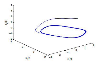
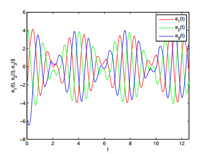
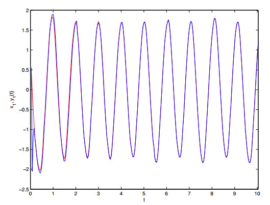
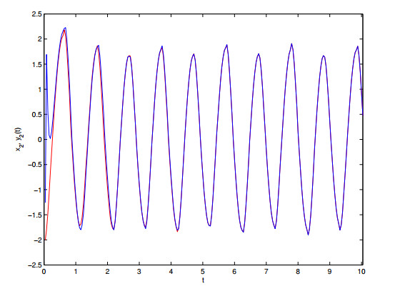
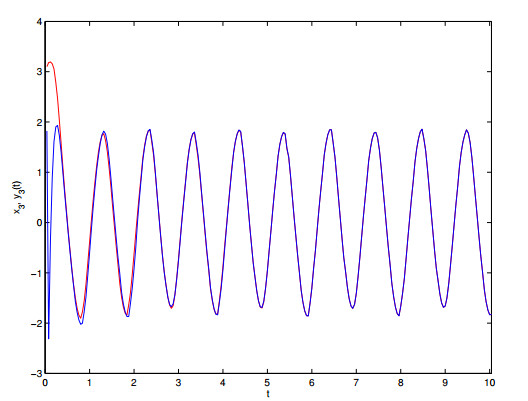
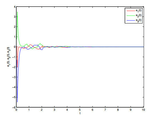
In this paper, synchronization of fractional-order memristive recurrent neural networks via aperiodically intermittent control is investigated. Considering the special properties of memristor neural network, differential inclusion theory is introduced. Similar to the aperiodically strategy of integer order, aperiodically intermittent control strategy of fractional order is proposed. Under the framework of Fillipov's solution, based on the intermittent strategy of fractional order systems and the properties Mittag-Leffler, sufficient criteria of aperiodically intermittent strategy are obtained by constructing appropriate Lyapunov functional. Some comparisons are given to demonstrate the advantages of aperiodically strategy. A simulation example is given to illustrate the derived conclusions.
Citation: Shuai Zhang, Yongqing Yang, Xin Sui, Yanna Zhang. Synchronization of fractional-order memristive recurrent neural networks via aperiodically intermittent control[J]. Mathematical Biosciences and Engineering, 2022, 19(11): 11717-11734. doi: 10.3934/mbe.2022545
In this paper, synchronization of fractional-order memristive recurrent neural networks via aperiodically intermittent control is investigated. Considering the special properties of memristor neural network, differential inclusion theory is introduced. Similar to the aperiodically strategy of integer order, aperiodically intermittent control strategy of fractional order is proposed. Under the framework of Fillipov's solution, based on the intermittent strategy of fractional order systems and the properties Mittag-Leffler, sufficient criteria of aperiodically intermittent strategy are obtained by constructing appropriate Lyapunov functional. Some comparisons are given to demonstrate the advantages of aperiodically strategy. A simulation example is given to illustrate the derived conclusions.

| [1] |
L. Chua, Memrisor-the missing circuit element, IEEE Trans. Circuit Theory, 18 (1971), 507–519. https://doi.org/10.1109/TCT.1971.1083337 doi: 10.1109/TCT.1971.1083337

|
| [2] |
L. Chua, S. Kang, Memristive devices and systems. Proc. IEEE, 64 (1976), 209–223. https://doi.org/10.1109/PROC.1976.10092 doi: 10.1109/PROC.1976.10092
|
| [3] |
D. Strukov, G. Snider, D. Stewart, R. Williams, The missing memristor found, Nature, 453 (2008), 80–83. https://doi.org/10.1038/nature06932 doi: 10.1038/nature06932
|
| [4] |
J. Tour, T. He, Electronics: The fourth element, Nature, 453 (2008), 42–43. https://doi.org/10.1038/453042a doi: 10.1038/453042a
|
| [5] |
W. Mao, Y. Liu, L. Ding, A. Safian, X. Liang, A new structured domain adversarial neural network for transfer fault diagnosis of rolling bearings under different working conditions, IEEE Trans. Instrum. Meas., 70 (2021), 1–13. https://doi.org/10.1109/TIM.2020.3038596 doi: 10.1109/TIM.2020.3038596
|
| [6] |
S. Wang, Z. Dou, D. Chen, H. Yu, Y. Li, P. Pan, Multimodal multiclass boosting and its application to cross-modal retrieval, Neurocomputing, 357 (2019), 11–23. https://doi.org/10.1016/j.neucom.2019.05.040 doi: 10.1016/j.neucom.2019.05.040
|
| [7] |
W. Mao, J. Wang, Z. Xue, An ELM-based model with sparse-weighting strategy for sequential data imbalance problem, Int. J. Mach. Learn. Cybern., 8 (2017), 1333–1345. https://doi.org/10.1007/s13042-016-0509-z doi: 10.1007/s13042-016-0509-z
|
| [8] |
S. Zhang, Y. Yang, L. Li, D. Wu, Quasi-synchronization of fractional-order complex-valued memristive recurrent neural networks with switching jumps mismatch, Neural Process Lett., 53 (2021), 865–-891. https://doi.org/10.1007/s11063-020-10342-4 doi: 10.1007/s11063-020-10342-4
|
| [9] |
Y. Shi, J. Cao, G. Chen, Exponential stability of complex-valued memristor-based neural networks with time-varying delays, Appl. Math. Comput., 313 (2017), 222–234. https://doi.org/10.1016/j.amc.2017.05.078 doi: 10.1016/j.amc.2017.05.078
|
| [10] |
X. Yang, D. Ho, Synchronization of delayed memristive neural networks: robust analysis approach, IEEE Trans. Cybern., 46 (2016), 3377–3387. https://doi.org/10.1109/TCYB.2015.2505903 doi: 10.1109/TCYB.2015.2505903
|
| [11] |
G. Zhang, Z. Zeng, Exponential stability for a class of memristive neural networks with mixed time-varying delays, Appl. Math. Comput., 321 (2018), 544–554. https://doi.org/10.1016/j.amc.2017.11.022 doi: 10.1016/j.amc.2017.11.022
|
| [12] |
M. Mehrabbeik, F. Parastesh, J. Ramadoss, K. Rajagopal, H. Namazi, S. Jafari, Synchronization and chimera states in the network of electrochemically coupled memristive Rulkov neuron maps, Math. Biosci. Eng., 18 (2021), 9394–9409. https://doi.org/10.3934/mbe.2021462 doi: 10.3934/mbe.2021462
|
| [13] |
T. Dong, X. Gong, T. Huang, Zero-Hopf bifurcation of a memristive synaptic Hopfield neural network with time delay, Neural Networks, 149 (2022), 146–156. https://doi.org/10.1016/j.neunet.2022.02.009 doi: 10.1016/j.neunet.2022.02.009
|
| [14] |
X. Yang, J. Cao, J. Liang, Exponential synchronization of memristive neural networks with delays: interval matrix method, IEEE Trans. Neural Networks Learn. Syst., 28 (2017), 1878–1888. https://doi.org/10.1109/TNNLS.2016.2561298 doi: 10.1109/TNNLS.2016.2561298
|
| [15] |
Y. Shi, J. Cao, G. Chen, Exponential stability of complex-valued memristor-based neural networks with time-varying delays, Appl. Math. Comput., 313 (2017), 222–234. https://doi.org/10.1016/j.amc.2017.05.078 doi: 10.1016/j.amc.2017.05.078
|
| [16] |
G. Zhang, Z. Zeng, J. Hu, New results on global exponential dissipativity analysis of memristive inertial neural networks with distributed time-varying delays, Neural Networks, 97 (2018), 183–191. https://doi.org/10.1016/j.neunet.2017.10.003 doi: 10.1016/j.neunet.2017.10.003
|
| [17] |
A. Wu, Y. Chen, Z. Zeng, Multi-mode function synchronization of memristive neural networks with mixed delays and parameters mismatch via event-triggered control, Inf. Sci., 572 (2021), 147–166. https://doi.org/10.1016/j.ins.2021.04.101 doi: 10.1016/j.ins.2021.04.101
|
| [18] |
X. Yang, J. Cao, J. Qiu, pth moment exponential stochastic synchronization of coupled memristor-based neural networks with mixed delays via delayed impulsive control, Neural Networks, 65 (2015), 80–91. https://doi.org/10.1016/j.neunet.2015.01.008 doi: 10.1016/j.neunet.2015.01.008
|
| [19] |
L. Zhang, Y. Yang, F. Wang, Projective synchronization of fractional-order memristive neural networks with switching jumps mismatch, Phys. A, 471 (2017), 402–415. https://doi.org/10.1016/j.physa.2016.12.030 doi: 10.1016/j.physa.2016.12.030
|
| [20] |
J. Zhang, Z. Lou, Y. Jia, W. Shao, Ground state of Kirchhoff type fractional Schrödinger equations with critical growth, J. Math. Anal. Appl., 462 (2018), 57–83. https://doi.org/10.1016/j.jmaa.2018.01.060 doi: 10.1016/j.jmaa.2018.01.060
|
| [21] |
B. Łupińska, E. Schmeidel, Analysis of some Katugampola fractional differential equations with fractional boundary conditions, Math. Biosci. Eng., 18 (2021), 1–19. https://doi.org/10.3934/mbe.2021359 doi: 10.3934/mbe.2021359
|
| [22] |
J. Zhang, J. Wang, Numerical analysis for Navier–Stokes equations with time fractional derivatives, Appl. Math. Comput., 30 (2022), 2747–2758. https://doi.org/10.1016/j.amc.2018.04.036 doi: 10.1016/j.amc.2018.04.036
|
| [23] |
F. Wang, Y. Yang, Quasi-synchronization for fractional-order delayed dynamical networks with heterogeneous nodes, Appl. Math. Comput., 339 (2018), 1–14. https://doi.org/10.1016/j.amc.2018.07.041 doi: 10.1016/j.amc.2018.07.041
|
| [24] | C. Huang, J. Cao, M. Xiao, A. Alsaedi, T. Hayat, Bifurcations in a delayed fractional complex-valued neural network, Appl. Math. Comput., 292 (2017), 210–227. https://doi.org/0.1016/j.amc.2018.07.041 |
| [25] |
L. Zhang, Y. Yang, F. Wang, Synchronization analysis of fractional-order neural networks with time-varying delays via discontinuous neuron activations, Neurocomputing, 275 (2018), 40–49. https://doi.org/10.1016/j.neucom.2017.04.056 doi: 10.1016/j.neucom.2017.04.056
|
| [26] |
C. Hu, H. Jiang, Special functions-based fixed-time estimation and stabilization for dynamic systems, IEEE Trans. Syst. Man Cybern., 5 (2022), 3251–3262. https://doi.org/10.1109/TSMC.2021.3062206 doi: 10.1109/TSMC.2021.3062206
|
| [27] |
S. Yang, C. Hu, J. Yu, H. Jiang, Finite-time cluster synchronization in complex-variable networks with fractional-order and nonlinear coupling, Neural Networks, 135 (2021), 212–224. https://doi.org/10.1016/j.neunet.2020.12.015 doi: 10.1016/j.neunet.2020.12.015
|
| [28] |
J. Fei, L. Liu, Real-time nonlinear model predictive control of active power filter using self-feedback recurrent fuzzy neural network estimator, IEEE Trans. Ind. Electron., 69 (2022), 8366–8376. https://doi.org/10.1109/TIE.2021.3106007 doi: 10.1109/TIE.2021.3106007
|
| [29] |
W. Sun, L. Peng, Observer-based robust adaptive control for uncertain stochastic Hamiltonian systems with state and input delays, Nonlinear Anal. Modell. Control, 19 (2014), 626–645. https://doi.org/10.15388/NA.2014.4.8 doi: 10.15388/NA.2014.4.8
|
| [30] |
S. Liu, J. Wang, Y. Zhou, M. Feckan, Iterative learning control with pulse compensation for fractional differential systems, Math. Slovaca, 68 (2018), 563–574. https://doi.org/10.1515/ms-2017-0125 doi: 10.1515/ms-2017-0125
|
| [31] |
M. Sabzalian, A. Mohammadzadeh, S. Lin, W. Zhang, Robust fuzzy control for fractional-order systems with estimated fraction-order, Nonlinear Dyn., 98 (2019), 2375–2385. https://doi.org/10.1007/s11071-019-05217-w doi: 10.1007/s11071-019-05217-w
|
| [32] |
Z. Wang, J. Fei, Fractional-order terminal sliding-mode control using self-evolving recurrent chebyshev fuzzy neural network for mems gyroscope, IEEE Trans. Fuzzy Syst., 30 (2022), 2747– 2758. https://doi.org/10.1109/TFUZZ.2021.3094717 doi: 10.1109/TFUZZ.2021.3094717
|
| [33] |
Y. Cao, S. Wang, Z. Guo, T. Huang, S. Wen, Synchronization of memristive neural networks with leakage delay and parameters mismatch via event-triggered control, Neural Networks, 119 (2019), 178–189. https://doi.org/10.1016/j.neunet.2019.08.011 doi: 10.1016/j.neunet.2019.08.011
|
| [34] |
X. Li, X. Yang, J. Cao, Event-triggered impulsive control for nonlinear delay systems, Automatica, 117 (2020), 108981. https://doi.org/10.1016/j.automatica.2020.108981 doi: 10.1016/j.automatica.2020.108981
|
| [35] |
X. Li, D. Peng, J. Cao, Lyapunov stability for impulsive systems via event-triggered impulsive control, IEEE Trans. Autom. Control, 65 (2020), 4908–4913. https://doi.org/10.1109/TAC.2020.2964558 doi: 10.1109/TAC.2020.2964558
|
| [36] |
H. Li, X. Gao, R. Li, Exponential stability and sampled-data synchronization of delayed complex-valued memristive neural networks, Neural Process Lett., 51 (2020), 193–209. https://doi.org/10.1007/s11063-019-10082-0 doi: 10.1007/s11063-019-10082-0
|
| [37] |
H. Fan, K. Shi, Y. Zhao, Global $\mu$-synchronization for nonlinear complex networks with unbounded multiple time delays and uncertainties via impulsive control, Phys. A, 599 (2022), 127484. https://doi.org/10.1016/j.physa.2022.127484 doi: 10.1016/j.physa.2022.127484
|
| [38] |
X. Li, D. Ho, J. Cao, Finite-time stability and settling-time estimation of nonlinear impulsive systems, Automatica, 99 (2019), 361–368. https://doi.org/10.1016/j.automatica.2018.10.024 doi: 10.1016/j.automatica.2018.10.024
|
| [39] |
S. Yang, C. Hu, J. Yu, H. Jiang, Exponential stability of fractional-order impulsive control systems with applications in synchronization, IEEE Trans. Cybern., 50 (2020), 3157–3168. https://doi.org/10.1109/TCYB.2019.2906497 doi: 10.1109/TCYB.2019.2906497
|
| [40] |
H. Fan, K. Shi, Y. Zhao, Pinning impulsive cluster synchronization of uncertain complex dynamical networks with multiple time-varying delays and impulsive effects, Phys. A, 587 (2022), 126534. https://doi.org/10.1016/j.physa.2021.126534 doi: 10.1016/j.physa.2021.126534
|
| [41] |
F. Wang, Y. Yang, Intermittent synchronization of fractional order coupled nonlinear systems based on a new differential inequality, Phys. A, 512 (2018), 142–152. https://doi.org/10.1016/j.physa.2018.08.023 doi: 10.1016/j.physa.2018.08.023
|
| [42] |
L. Zhang, Y. Yang, F. Wang, Lag synchronization for fractional-order memristive neural networks via period intermittent control, Nonlinear Dyn., 89 (2017), 367–381. https://doi.org/10.1007/s11071-017-3459-4 doi: 10.1007/s11071-017-3459-4
|
| [43] |
C. Hu, H. He, H. Jiang, Synchronization of complex-valued dynamic networks with intermittently adaptive coupling: A direct error method, Automatica, 112 (2020), 108675. https://doi.org/10.1016/j.automatica.2019.108675 doi: 10.1016/j.automatica.2019.108675
|
Figures(10)

Shuai Zhang, Yongqing Yang, Xin Sui, Yanna Zhang. Synchronization of fractional-order memristive recurrent neural networks via aperiodically intermittent control[J]. Mathematical Biosciences and Engineering, 2022, 19(11): 11717-11734. doi: 10.3934/mbe.2022545


 DownLoad: