Automatic segmentation of breast cancer histological images based on dual-path feature extraction network

Xi Lu; Xuedong Zhu; Xi Lu; Xuedong Zhu

doi:10.3934/mbe.2022519

Mathematical Biosciences and Engineering

2022, Volume 19, Issue 11: 11137-11153. doi: 10.3934/mbe.2022519

Previous Article Next Article

Research article

Automatic segmentation of breast cancer histological images based on dual-path feature extraction network

Xi Lu ^,,
Xuedong Zhu

School of Mechanical Engineering, Southeast University, Nanjing 211189, China

Academic Editor: Weining Wu

Received: 07 May 2022 Revised: 14 July 2022 Accepted: 18 July 2022 Published: 03 August 2022

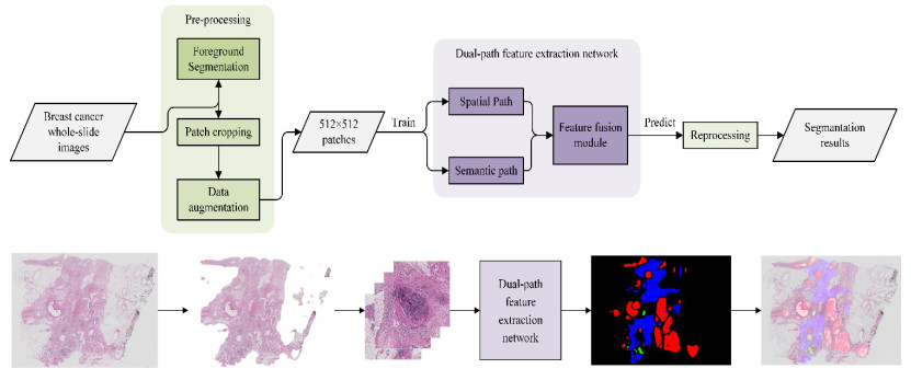
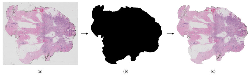
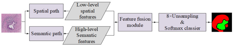
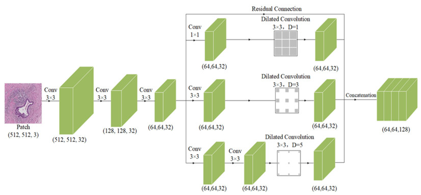
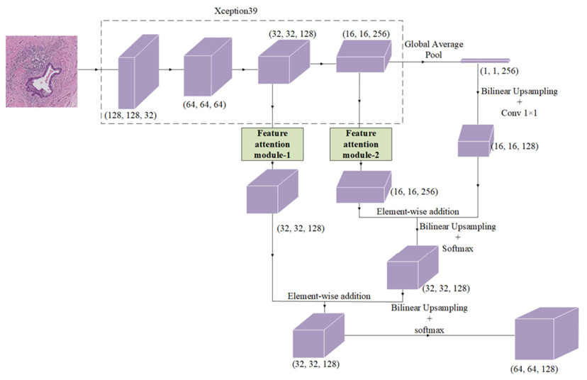
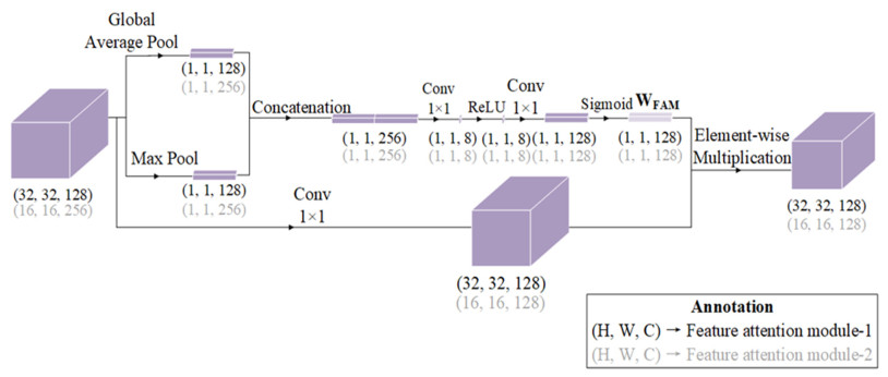
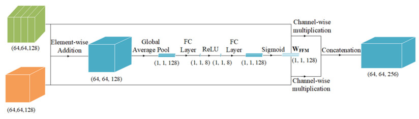
The traditional manual breast cancer diagnosis method of pathological images is time-consuming and labor-intensive, and it is easy to be misdiagnosed. Computer-aided diagnosis of WSIs gradually comes into people*s sight. However, the complexity of high-resolution breast cancer pathological images poses a great challenge to automatic diagnosis, and the existing algorithms are often difficult to balance the accuracy and efficiency. In order to solve these problems, this paper proposes an automatic image segmentation method based on dual-path feature extraction network for breast pathological WSIs, which has a good segmentation accuracy. Specifically, inspired by the concept of receptive fields in the human visual system, dilated convolutional networks are introduced to encode rich contextual information. Based on the channel attention mechanism, a feature attention module and a feature fusion module are proposed to effectively filter and combine the features. In addition, this method uses a light-weight backbone network and performs pre-processing on the data, which greatly reduces the computational complexity of the algorithm. Compared with the classic models, it has improved accuracy and efficiency and is highly competitive.
- semantic segmentation,
- breast cancer,
- whole-slide image,
- feature extraction,
- computer-aided diagnosis,
- deep learning
Citation: Xi Lu, Xuedong Zhu. Automatic segmentation of breast cancer histological images based on dual-path feature extraction network[J]. Mathematical Biosciences and Engineering, 2022, 19(11): 11137-11153. doi: 10.3934/mbe.2022519

Related Papers:

Abstract

The traditional manual breast cancer diagnosis method of pathological images is time-consuming and labor-intensive, and it is easy to be misdiagnosed. Computer-aided diagnosis of WSIs gradually comes into people*s sight. However, the complexity of high-resolution breast cancer pathological images poses a great challenge to automatic diagnosis, and the existing algorithms are often difficult to balance the accuracy and efficiency. In order to solve these problems, this paper proposes an automatic image segmentation method based on dual-path feature extraction network for breast pathological WSIs, which has a good segmentation accuracy. Specifically, inspired by the concept of receptive fields in the human visual system, dilated convolutional networks are introduced to encode rich contextual information. Based on the channel attention mechanism, a feature attention module and a feature fusion module are proposed to effectively filter and combine the features. In addition, this method uses a light-weight backbone network and performs pre-processing on the data, which greatly reduces the computational complexity of the algorithm. Compared with the classic models, it has improved accuracy and efficiency and is highly competitive.

References

[1]	H. Sung, J. Ferlay, R. L. Siegel, M. Laversanne, I. Soerjomataram, A. Jemal, et al., Global cancer statistics 2020: GLOBOCAN estimates of incidence and mortality worldwide for 36 cancers in 185 countries, CA Cancer J. Clin., 71 (2021), 209–249. https://doi.org/10.3322/caac.21660 doi: 10.3322/caac.21660
[2]	A. Das, M. S. Nair, S. D. Peter, Computer-aided histopathological image analysis techniques for automated nuclear atypia scoring of breast cancer: a review, J. Dig. Imaging, 33 (2020), 1–31. https://doi.org/10.1007/s10278-019-00295-z doi: 10.1007/s10278-020-00318-0
[3]	L. He, R. Long, S. Antani, G. R. Thoma, Histology image analysis for carcinoma detection and grading, Comput. Methods Prog. Biomed., 107 (2012), 538–556. https://doi.org/10.1016/j.cmpb.2011.12.007 doi: 10.1016/j.cmpb.2011.12.007
[4]	L. Dalton, Artificial intelligence grading of breast cancer: A study of ensemble learning, Lab. Investig., 102 (2022), 107–108.
[5]	J. G. Elmore, G. M. Longton, P. A. Carney, B. M. Geller, T. Onega, A. N. A. Tosteson, et al., Diagnostic concordance among pathologists interpreting breast biopsy specimens, JAMA, 313 (2015), 1122–1132. https://doi.org/10.1001/jama.2015.1405 doi: 10.1001/jama.2015.1405
[6]	K. E. Lindquist, C. Ciornei, S. Westbom-Fremer, I. Gudinaviciene, A. Ehinger, N. Mylona, et al., Difficulties in diagnostics of lung tumours in biopsies: an interpathologist concordance study evaluating the international diagnostic guidelines, J. Clin. Pathol., 75 (2022), 302–309. http://dx.doi.org/10.1136/jclinpath-2020-207257 doi: 10.1136/jclinpath-2020-207257
[7]	C. Merkouri, D. Grapsa, I. Tourkantonis, I. Gkiozos, A. Charpidou, G. Tournas, et al. Cytology-histology concordance for diagnosis, histological subtyping and molecular profiling of lung cancer, J. Thorac. Oncol., 16 (2021), S463. https://doi.org/10.1016/j.jtho.2021.01.794 doi: 10.1016/j.jtho.2021.01.794
[8]	V. K. Singh, H. A. Rashwan, M. Abdel-Nasser, F. Akram, R. Haffar, N. Pandey, et al., A computer-aided diagnosis system for breast cancer molecular subtype prediction in mammographic images, State Art Neural Networks Their Appl., 1 (2021), 153–178. https://doi.org/10.1016/B978-0-12-819740-0.00008-5 doi: 10.1016/B978-0-12-819740-0.00008-5
[9]	M. Perumal, A research on computer aided detection system for women breast cancer diagnosis from digital mammographic images, Int. J. Recent Technol. Eng., 2021 (2021). https://doi.org/10.35940/ijrte.B1169.0982S1119 doi: 10.35940/ijrte.B1169.0982S1119
[10]	S. Naik, S. Doyle, S. Agner, A. Madabhushi, M. Feldman, J. Tomaszewski, Automated gland and nuclei segmentation for grading of prostate and breast cancer histopathology, in 2008 5th IEEE International Symposium on Biomedical Imaging: From Nano to Macro, (2008). https://doi.org/10.1109/ISBI.2008.4540988
[11]	C. Jung, C. Kim, Segmenting clustered nuclei using H-minima transform-based marker extraction and contour parameterization, IEEE Trans. Biomed. Eng., 57 (2010), 2600–2604. https://doi.org/10.1109/TBME.2010.2060336 doi: 10.1109/TBME.2010.2060336
[12]	M. Kowal, P. Filipczuk, A. Obuchowicz, J. Korbicz, R. Monczak, Computer-aided diagnosis of breast cancer based on fine needle biopsy microscopic images, Comput. Biol. Med., 43 (2013), 1563–1572. https://doi.org/10.1016/j.compbiomed.2013.08.003 doi: 10.1016/j.compbiomed.2013.08.003
[13]	A. D. Belsare, M. M. Mushrif, M. A. Pangarkar, N. Meshram, Breast histopathology image segmentation using spatio-colour-texture based graph partition method, J. Microscopy, 262 (2016), 260–273. https://doi.org/10.1111/jmi.12361 doi: 10.1111/jmi.12361
[14]	Z. Senousy, M. M. Abdelsamea, M. M. Mohamed, M. M. Gaber, 3E-Net: Entropy-based elastic ensemble of deep convolutional neural networks for grading of invasive breast carcinoma histopathological microscopic images, Entropy, 23 (2021), 620. https://doi.org/10.3390/e23050620 doi: 10.3390/e23050620
[15]	Y. Yari, T. V. Nguyen, H. T. Nguyen, Deep learning applied for histological diagnosis of breast cancer, IEEE Access, 8 (2020), 162463–162448. https://doi.org/10.1109/ACCESS.2020.3021557 doi: 10.1109/ACCESS.2020.3021557
[16]	D. C. Ciresan, A. Giusti, L. M. Gambardella, J. Schmidhuber, Mitosis detection in breast cancer histology images with deep neural networks, in International Conference on Medical Image Computing and Computer-Assisted Intervention, (2013). https://doi.org/10.1007/978-3-642-40763-5_51
[17]	G. Litjens, C. I. Sánchez, N. Timofeeva, M. Hermsen, I. Nagtegaal, I. Kovacs, et al., Deep learning as a tool for increased accuracy and efficiency of histopathological diagnosis, Sci. Rep., 6 (2016), 26286. https://doi.org/10.1038/srep26286 doi: 10.1038/srep26286
[18]	O. Ronneberger, P. Fischer, T. Brox, U-Net: Convolutional networks for biomedical image segmentation, in International Conference on Medical Image Computing and Computer-Assisted Intervention, (2015). https://doi.org/10.1007/978-3-319-24574-4_28
[19]	D. J. Ho, D. Yarlagadda, T. M. D'Alfonso, M. G. Hanna, A. Grabenstetter, P. Ntiamoah, et al., Deep multi-magnification networks for multi-class breast cancer image segmentation, Comput. Med. Imaging Graphics, 88 (2021), 101866. https://doi.org/10.1016/j.compmedimag.2021.101866 doi: 10.1016/j.compmedimag.2021.101866
[20]	I. Anand, H. Negi, D. Kumar, M. Mittal, T. Kim, S. Roy, Residual U-network for breast tumor segmentation from magnetic resonance images, Comput. Mater. Continua, 67 (2021), 3107–3127. http://doi.org/10.32604/cmc.2021.014229 doi: 10.32604/cmc.2021.014229
[21]	L. C. Chen, G. Papandreou, I. Kokkinos, K. Murphy, A. L. Yuille, DeepLab: Semantic image segmentation with deep convolutional nets, atrous convolution, and fully connected CRFs, IEEE Trans. Pattern Anal. Mach. Intell., 40 (2018), 834–848. https://doi.org/10.1109/TPAMI.2017.2699184 doi: 10.1109/TPAMI.2017.2699184
[22]	J. Wang, X. Liu, Medical image recognition and segmentation of pathological slices of gastric cancer based on Deeplab v3+ neural network, Comput. Methods Prog. Biomed., 207 (2021), 106210. https://doi.org/10.1016/j.cmpb.2021.106210 doi: 10.1016/j.cmpb.2021.106210
[23]	C. Yu, J. Wang, C. Peng, C. Gao, G. Yu, N. Sang, BiSeNet: Bilateral segmentation network for real-time semantic segmentation, in Proceedings of the European Conference on Computer Vision (ECCV), (2018).
[24]	G. Aresta, T. Araújo, S. Kwok, S. S. Chennamsetty, M. Safwan, V. Alex, et al., BACH: Grand challenge on breast cancer histology images, Med. Image Anal., 56 (2019), 122–139. https://doi.org/10.1016/j.media.2019.05.010 doi: 10.1016/j.media.2019.05.010
[25]	S. Krishnamurthy, K. Mathews, S. McClure, M. Murray, M. Gilcrease, C. Albarracin, et al., Multi-institutional comparison of Whole slide digital imaging and optical microscopy for interpretation of hematoxylin-eosin-stained breast tissue sections, Arch. Pathol. Lab. Med., 137 (2013), 1733–1739. https://doi.org/10.5858/arpa.2012-0437-OA doi: 10.5858/arpa.2012-0437-OA
[26]	A. Canziani, A. Paszke, E. Culurciello, An analysis of deep neural network models for practical applications, preprint, arXiv: 1605.07678.
[27]	S. Liu, D. Huang, Y. Wang, Receptive field block net for accurate and fast object detection, in Proceedings of the European Conference on Computer Vision (ECCV), (2018).
[28]	F. Chollet, Xception: Deep learning with depthwise separable convolutions, in 2017 IEEE Conference on Computer Vision and Pattern Recognition (CVPR), (2017).
[29]	J. Hu, L. Shen, G. Sun, Squeeze-and-excitation networks, in Proceedings of the IEEE Conference on Computer Vision and Pattern Recognition (CVPR), (2018).
[30]	A. Buslaev, V. I. Iglovikov, E. Khvedchenya, A. Parinov, M. Druzhinin, A. A. Kalinin, Albumentations: fast and flexible image augmentations, Information, 11 (2020), 125. https://doi.org/10.3390/info11020125 doi: 10.3390/info11020125
[31]	S. Mantrala, P. S. Ginter, A. Mitkar, S. Joshi, H. Prabhala, V. Ramachandra, Concordance in breast cancer grading by artificial intelligence on whole slide images compares with a multi-Institutional cohort of breast pathologists, Arch. Pathol. Lab. Med., 2022 (2022), forthcoming. https://doi.org/10.5858/arpa.2021-0299-OA

Reader Comments

Your name:*

Email:*
© 2022 the Author(s), licensee AIMS Press. This is an open access article distributed under the terms of the Creative Commons Attribution License (http://creativecommons.org/licenses/by/4.0)