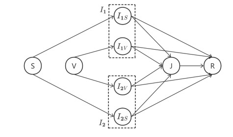
Coinfection is the process of an infection of a single host with two or more pathogen variants or with two or more distinct pathogen species, which often threatens public health and the stability of economies. In this paper, we propose a novel two-strain epidemic model characterizing the co-evolution of coinfection and voluntary vaccination strategies. In the framework of evolutionary vaccination, we design two game rules, the individual-based risk assessment (IB-RA) updated rule, and the strategy-based risk assessment (SB-RA) updated rule, to update the vaccination policy. Through detailed numerical analysis, we find that increasing the vaccine effectiveness and decreasing the transmission rate effectively suppress the disease prevalence, and moreover, the outcome of the SB-RA updated rule is more encouraging than those results of the IB-RA rule for curbing the disease transmission. Coinfection complicates the effects of the transmission rate of each strain on the final epidemic sizes.
Citation: Kelu Li, Junyuan Yang, Xuezhi Li. Effects of co-infection on vaccination behavior and disease propagation[J]. Mathematical Biosciences and Engineering, 2022, 19(10): 10022-10036. doi: 10.3934/mbe.2022468
Coinfection is the process of an infection of a single host with two or more pathogen variants or with two or more distinct pathogen species, which often threatens public health and the stability of economies. In this paper, we propose a novel two-strain epidemic model characterizing the co-evolution of coinfection and voluntary vaccination strategies. In the framework of evolutionary vaccination, we design two game rules, the individual-based risk assessment (IB-RA) updated rule, and the strategy-based risk assessment (SB-RA) updated rule, to update the vaccination policy. Through detailed numerical analysis, we find that increasing the vaccine effectiveness and decreasing the transmission rate effectively suppress the disease prevalence, and moreover, the outcome of the SB-RA updated rule is more encouraging than those results of the IB-RA rule for curbing the disease transmission. Coinfection complicates the effects of the transmission rate of each strain on the final epidemic sizes.

| [1] |
S. Basu, G. B. Chapman, A. P. Galvani, Integrating epidemiology, psychology, and economics to achieve hpv vaccination targets, Proc. Natl. Acad. Sci., 105 (2008), 19018–19023. https://doi.org/10.1073/pnas.0808114105 doi: 10.1073/pnas.0808114105

|
| [2] |
C. T. Bauch, A. P. Galvani, D. J. D. Earn, Group interest versus self-interest in smallpox vaccination policy, Proc. Natl. Acad. Sci., 100 (2003), 10564–10567. https://doi.org/10.1073/pnas.1731324100 doi: 10.1073/pnas.1731324100
|
| [3] |
C. T. Bauch, D. J. D. Earn, Vaccination and the theory of games, Proc. Natl. Acad. Sci., 101 (2004), 13391–13394. https://doi.org/10.1073/pnas.0403823101 doi: 10.1073/pnas.0403823101
|
| [4] |
C. T. Bauch, Imitation dynamics predict vaccinating behaviour, Proc. R. Soc. B, 272 (2005), 1669–1675. https://doi.org/10.1098/rspb.2005.3153 doi: 10.1098/rspb.2005.3153
|
| [5] |
Z. Wang, Y. Moreno, S. Boccaletti, M. Perc, Vaccination and epidemics in networked populations–an introduction, Chaos Solitons Fractals, 103 (2017), 177–183. https://doi.org/10.1016/j.chaos.2017.06.004 doi: 10.1016/j.chaos.2017.06.004
|
| [6] |
K. Kuga, J. Tanimoto, Impact of imperfect vaccination and defense against contagion on vaccination behavior in complex networks, J. Stat. Mech. Theory Exp., 2018 (2018), 113402. https://doi.org/10.1088/1742-5468/aae84f doi: 10.1088/1742-5468/aae84f
|
| [7] |
R. Vardavas, R. Breban, S. Blower, Can influenza epidemics be prevented by voluntary vaccination?, PLoS Comput. Biol., 3 (2007), e85. https://doi.org/10.1371/journal.pcbi.0030085 doi: 10.1371/journal.pcbi.0030085
|
| [8] |
A. Cardillo, C. Reyes-Suárez, F. Naranjo, J. Gómez-Gardenes, Evolutionary vaccination dilemma in complex networks, Phys. Rev. E, 288 (2013), 032803. https://doi.org/10.1103/PhysRevE.88.032803 doi: 10.1103/PhysRevE.88.032803
|
| [9] |
B. Wu, F. Fu, L. Wang, Imperfect vaccine aggravates the long-standing dilemma of voluntary vaccination, PloS One, 6 (2011), e20577. https://doi.org/10.1371/journal.pone.0020577 doi: 10.1371/journal.pone.0020577
|
| [10] |
Z. Wang, C. T. Bauch, S. Bhattacharyya, A. d'Onofrio, P. Manfredi, M. Perc, et al., Statistical physics of vaccination, Phys. Rep., 664 (2016), 1–113. https://doi.org/10.1016/j.physrep.2016.10.006 doi: 10.1016/j.physrep.2016.10.006
|
| [11] |
A. Deka, S. Bhattacharyya, Game dynamic model of optimal budget allocation under individual vaccination choice, J. Theor. Biol., 470 (2019), 108–118. https://doi.org/10.1016/j.jtbi.2019.03.014 doi: 10.1016/j.jtbi.2019.03.014
|
| [12] |
G. B. Chapman, M. Li, J. Vietri, Y. Ibuka, D. Thomas, H. Yoon, et al., Using game theory to examine incentives in influenza vaccination behavior, Psychol. Sci., 23 (2012), 1008–1015. https://doi.org/10.1177/0956797612437606 doi: 10.1177/0956797612437606
|
| [13] |
G. Ichinose, T. Kurisaku, Positive and negative effects of social impact on evolutionary vaccination game in networks, Physica A: Statistical Mechanics and its Applications, 468 (2017), 84–90. https://doi.org/10.1016/j.physa.2016.10.017 doi: 10.1016/j.physa.2016.10.017
|
| [14] |
K. M. A. Kabir, K. Kuga, J. Tanimoto, Analysis of sir epidemic model with information spreading of awareness, Chaos Solitons Fractals, 119 (2019), 118–125. https://doi.org/10.1016/j.chaos.2018.12.017 doi: 10.1016/j.chaos.2018.12.017
|
| [15] |
K. Kuga, J. Tanimoto, imperfect vaccination or defense against contagion?, Journal of Statistical Mechanics: Theory and Experiment, 2018 (2018), 023407. https://doi.org/10.1088/1742-5468/aaac3c doi: 10.1088/1742-5468/aaac3c
|
| [16] |
M. Alam, M. Tanaka, J. Tanimoto, A game theoretic approach to discuss the positive secondary effect of vaccination scheme in an infinite and well-mixed population, Chaos Solitons Fractals, 125 (2019), 201–213. https://doi.org/10.1016/j.chaos.2019.05.031 doi: 10.1016/j.chaos.2019.05.031
|
| [17] |
M. Alam, K. Kabir, J. Tanimoto, Based on mathematical epidemiology and evolutionary game theory, which is more effective: quarantine or isolation policy?, J. Stat. Mech. Theory Exp., 2020 (2020), 033502. https://doi.org/10.1088/1742-5468/ab75ea doi: 10.1088/1742-5468/ab75ea
|
| [18] |
M. Arefin, K. Kabir, J. Tanimoto, A mean-field vaccination game scheme to analyze the effect of a single vaccination strategy on a two-strain epidemic spreading, J. Stat. Mech. Theory Exp., 2020 (2020), 033501. https://doi.org/10.1088/1742-5468/ab74c6 doi: 10.1088/1742-5468/ab74c6
|
| [19] |
K. Kabir, M. Jusup, J. Tanimoto, Behavioral incentives in a vaccination-dilemma setting with optional treatment, Phys. Rev. E, 100 (2019), 062402. https://doi.org/10.1103/PhysRevE.100.062402 doi: 10.1103/PhysRevE.100.062402
|
| [20] |
J. Huang, J. Wang, C. Xia, Role of vaccine efficacy in the vaccination behavior under myopic update rule on complex networks, Chaos Solitons Fractals, 130 (2020), 109425. https://doi.org/10.1016/j.chaos.2019.109425 doi: 10.1016/j.chaos.2019.109425
|
| [21] |
T. Krueger, K. Gogolewski, M. Bodych, A. Gambin, G. Giordano, S. Cuschieri, et al., Risk assessment of covid-19 epidemic resurgence in relation to sars-cov-2 variants and vaccination passes, Commun. Med., 2 (2022), 1–14. https://doi.org/10.1038/s43856-022-00084-w.eCollection2022 doi: 10.1038/s43856-022-00084-w.eCollection2022
|
| [22] |
D. Gao, T. Porco, S. Ruan, Coinfection dynamics of two diseases in a single host population, J. Math. Anal. Appl., 442 (2016), 171–188. https://doi.org/10.1016/j.jmaa.2016.04.039 doi: 10.1016/j.jmaa.2016.04.039
|
| [23] |
A. Elaiw, A. Agha, S. Azoz, E. Ramadan, Global analysis of within-host sars-cov-2/hiv coinfection model with latency, Eur. Phys. J. Plus, 137 (2022), 1–22. https://doi.org/10.1140/epjp/s13360-022-02387-2 doi: 10.1140/epjp/s13360-022-02387-2
|
| [24] |
I, Hezam, A, Foul, A, Alrasheedi, A dynamic optimal control model for covid-19 and cholera co-infection in yemen, Adv. Differ. Equations, 2021 (2021), 1–30. https://doi.org/10.1186/s13662-021-03271-6 doi: 10.1186/s13662-021-03271-6
|
| [25] |
M. Newman, C. Ferrario, Interacting epidemics and coinfection on contact networks, PloS One, 8 (2013), e71321. https://doi.org/10.1371/journal.pone.0071321 doi: 10.1371/journal.pone.0071321
|
| [26] |
S. Osman, O. Makinde, A mathematical model for coinfection of listeriosis and anthrax diseases, Int. J. Math. Math. Sci., 2018 (2018). https://doi.org/10.1155/2018/1725671 doi: 10.1155/2018/1725671
|
| [27] |
M. Martcheva, S. Pilyugin, The role of coinfection in multidisease dynamics. SIAM J. Appl. Math., 66 (2006), 843–872. https://doi.org/10.1137/040619272 doi: 10.1137/040619272
|
| [28] |
X. Li, S. Gao, Y. Fu, M. Martcheva, Modeling and research on an immuno-epidemiological coupled system with coinfection, Bull. Math. Biol., 83 (2021), 1–42. https://doi.org/10.1007/s11538-021-00946-9 doi: 10.1007/s11538-021-00946-9
|
| [29] |
J. Sanz, C. Xia, S. Meloni, Y. Moreno, Dynamics of interacting diseases, Phys. Rev. X, 4 (2014), 041005. https://doi.org/10.1103/PhysRevX.4.041005 doi: 10.1103/PhysRevX.4.041005
|
| [30] | Centers for disease control and prevention, Vaccine effectiveness: How well do flu vaccines work?, 2021. Available from: https://www.cdc.gov/flu/vaccines-work/vaccineeffect.htm. |
| [31] | World Health Organization, Influenza (seasonal), 2018. Available from: https://www.who.int/news-room/fact-sheets/detail/influenza-(seasonal). |
| [32] |
P. Van den Driessche, J. Watmough, Reproduction numbers and sub-threshold endemic equilibria for compartmental models of disease transmission, Math. Biosci., 180 (2002), 29–48. https://doi.org/10.1016/S0025-5564(02)00108-6 doi: 10.1016/S0025-5564(02)00108-6
|
| [33] |
F. Fu, D. Rosenbloom, L. Wang, M. Nowak, Imitation dynamics of vaccination behaviour on social networks, Proc. R. Soc. B, 278 (2011), 42–49. https://doi.org/10.1098/rspb.2010.1107 doi: 10.1098/rspb.2010.1107
|
| [34] |
E. Fukuda, S. Kokubo, J. Tanimoto, Z. Wang, A. Hagishima, N. Ikegaya, Risk assessment for infectious disease and its impact on voluntary vaccination behavior in social networks, Chaos Solitons Fractals, 68 (2014), 1–9. https://doi.org/10.1016/j.chaos.2014.07.004 doi: 10.1016/j.chaos.2014.07.004
|


Figures(3) / Tables(2)

Kelu Li, Junyuan Yang, Xuezhi Li. Effects of co-infection on vaccination behavior and disease propagation[J]. Mathematical Biosciences and Engineering, 2022, 19(10): 10022-10036. doi: 10.3934/mbe.2022468


 DownLoad: