Dynamic graph Conv-LSTM model with dynamic positional encoding for the large-scale traveling salesman problem

Yang Wang; Zhibin Chen; Yang Wang; Zhibin Chen

doi:10.3934/mbe.2022452

Mathematical Biosciences and Engineering

2022, Volume 19, Issue 10: 9730-9748. doi: 10.3934/mbe.2022452

Previous Article Next Article

Research article

Dynamic graph Conv-LSTM model with dynamic positional encoding for the large-scale traveling salesman problem

Yang Wang ,
Zhibin Chen ^,

Department of Mathematics, Kunming University of Science and Technology, Kunming 650093, China

Academic Editor: Runzhang Xu

Received: 19 May 2022 Revised: 20 June 2022 Accepted: 23 June 2022 Published: 04 July 2022

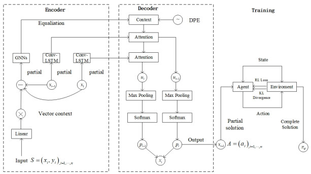
Recent research has showen that deep reinforcement learning (DRL) can be used to design better heuristics for the traveling salesman problem (TSP) on the small scale, but does not do well when generalized to large instances. In order to improve the generalization ability of the model when the nodes change from small to large, we propose a dynamic graph Conv-LSTM model (DGCM) to the solve large-scale TSP. The noted feature of our model is the use of a dynamic encoder-decoder architecture and a convolution long short-term memory network, which enable the model to capture the topological structure of the graph dynamically, as well as the potential relationships between nodes. In addition, we propose a dynamic positional encoding layer in the DGCM, which can improve the quality of solutions by providing more location information. The experimental results show that the performance of the DGCM on the large-scale TSP surpasses the state-of-the-art DRL-based methods and yields good performance when generalized to real-world datasets. Moreover, our model compares favorably to heuristic algorithms and professional solvers in terms of computational time.

Keywords:

Citation: Yang Wang, Zhibin Chen. Dynamic graph Conv-LSTM model with dynamic positional encoding for the large-scale traveling salesman problem[J]. Mathematical Biosciences and Engineering, 2022, 19(10): 9730-9748. doi: 10.3934/mbe.2022452

Related Papers:

[1]	Hui Li, Mengyao Zhang, Chenbo Zeng . Circular Jaccard distance based multi-solution optimization for traveling salesman problems. Mathematical Biosciences and Engineering, 2022, 19(5): 4458-4480. doi: 10.3934/mbe.2022206
[2]	Teng Fei, Xinxin Wu, Liyi Zhang, Yong Zhang, Lei Chen . Research on improved ant colony optimization for traveling salesman problem. Mathematical Biosciences and Engineering, 2022, 19(8): 8152-8186. doi: 10.3934/mbe.2022381
[3]	Ruiping Yuan, Jiangtao Dou, Juntao Li, Wei Wang, Yingfan Jiang . Multi-robot task allocation in e-commerce RMFS based on deep reinforcement learning. Mathematical Biosciences and Engineering, 2023, 20(2): 1903-1918. doi: 10.3934/mbe.2023087
[4]	Kun Yu, Mingxu Huang, Shuaizheng Chen, Chaolu Feng, Wei Li . GSEnet: feature extraction of gene expression data and its application to Leukemia classification. Mathematical Biosciences and Engineering, 2022, 19(5): 4881-4891. doi: 10.3934/mbe.2022228
[5]	Keruo Jiang, Zhen Huang, Xinyan Zhou, Chudong Tong, Minjie Zhu, Heshan Wang . Deep belief improved bidirectional LSTM for multivariate time series forecasting. Mathematical Biosciences and Engineering, 2023, 20(9): 16596-16627. doi: 10.3934/mbe.2023739
[6]	Kunli Zhang, Bin Hu, Feijie Zhou, Yu Song, Xu Zhao, Xiyang Huang . Graph-based structural knowledge-aware network for diagnosis assistant. Mathematical Biosciences and Engineering, 2022, 19(10): 10533-10549. doi: 10.3934/mbe.2022492
[7]	Zhiwen Hou, Fanliang Bu, Yuchen Zhou, Lingbin Bu, Qiming Ma, Yifan Wang, Hanming Zhai, Zhuxuan Han . DyCARS: A dynamic context-aware recommendation system. Mathematical Biosciences and Engineering, 2024, 21(3): 3563-3593. doi: 10.3934/mbe.2024157
[8]	Shixuan Yao, Xiaochen Liu, Yinghui Zhang, Ze Cui . An approach to solving optimal control problems of nonlinear systems by introducing detail-reward mechanism in deep reinforcement learning. Mathematical Biosciences and Engineering, 2022, 19(9): 9258-9290. doi: 10.3934/mbe.2022430
[9]	Yun Hu, Qianqian Duan . Solving the TSP by the AALHNN algorithm. Mathematical Biosciences and Engineering, 2022, 19(4): 3427-3448. doi: 10.3934/mbe.2022158
[10]	Bowen Ding, Zhaobin Ma, Shuoyan Ren, Yi Gu, Pengjiang Qian, Xin Zhang . A genetic algorithm with two-step rank-based encoding for closed-loop supply chain network design. Mathematical Biosciences and Engineering, 2022, 19(6): 5925-5956. doi: 10.3934/mbe.2022277

Abstract

1. Introduction

A wide variety of heat-transfer problems applied to Newtonian fluids flow in bounded conduits of cylindrical or parallel-plate geometries with negligible axial conduction has been successfully reduced and known as the Graetz problem ^[1,2]. Multi-stream or multiphase systems, however, are fundamentally different since conjugated boundary conditions must be coupled at the boundaries, referred to as conjugated Graetz problems ^[3,4], which were solved analytically by means of an orthogonal expansion technique ^[5,6] with the eigenfunction expansion in terms of the extended power series. Extension to markedly increased applications of practical processes with recycle-effect concept is possible. It's been widely used in separation, fermentation, and polymerization such as distillation ^[7], extraction ^[8], loop reactors ^[9], air-lift reactor ^[10], draft-tube bubble column ^[11], mass exchanger ^[12], and thermal diffusion column ^[13].

Many materials of food, polymeric systems, biological process, pulp and paper suspensions ^[14] with high molecular weight in processing industries exhibit a range of non-Newtonian fluid behavioral features and display shear-thinning and/or shear thickening behavior ^[15,16]. Those non-Newtonian fluids can be treated as the laminar flow conditions with negligible viscoelastic effects based on their high viscosity levels in the appropriate shear rate range ^[17]. Therefore, the analytical solution could be analogously obtained under the similar mathematical treatment when dealing with Newtonian fluids. A considerable body of literature has shown the practical feasibility of solving the power-law model of non-Newtonian flows by LBM (Lattice Boltzmann Method). It is also devoted to studying the non-Newtonian behavior with shear-thinning and shear-thickening liquids on sedimentation ^[18,19] and flows over a heated cylinder ^[20], an inclined square ^[21], cylinder ^[22] and various shapes ^[23]. Furthermore, the heat-transfer responses to the distributions of the conduit wall and fluid temperature are two major concerns in investigating the heat-transfer efficiency improvement under different kinds of boundary conditions which can be detected at the conduit wall. Two cases of the uniform wall temperature (Dirichlet problem) ^[24,25] and uniform heat flux (Neumann problem) ^[26,27] were processed in the application of engineering field, in general. Recently, a non-trivial amount of research use metal foams of PCMs (phase change materials) and nanoparticles of NEPCMs (nano-encapsulated phase change materials) to enhance heat transfer properties in some applications regarding constant heat load, transient, or cyclic loads. Thermal and energy storage managements of crucial importance of systems were investigated within the thermal performance given variable heat loads ^[28] and non-uniform magnetic sources ^[29], as well as thermal benefit of NEPCMs nanoparticles in microchannels that considers forced convection ^[30] and natural convection flow ^[31,32]. However, the well-known case of sinusoidal wall heat flux distribution ^[33] of non-uniform heating was the simplest model of period heating within the convective heat-transfer problems in the periodic ^[34] and circumferentially ^[35] heating systems. It's been investigated by many researchers to design the cooling tubes in nuclear reactors ^[36].

The present study is an extension of our previous work ^[37] to apply the system of non-Newtonian fluids for the conjugated Graetz problem where the power-law index of the shearing-thinning aqueous polymer solutions were given. Though the phenomenon of heat transfer in the present study could be drawn parallel comparison, in similar sense, with that of heat-transfer mechanism in our previous work ^[37], the manners of non-Newtonian fluids with the convective heat transfer are somehow different. It's actually affected by the velocity profile of shear-thinning fluid. A power-law fluid flowing through a double-pass laminar countercurrent-flow concentric-tube heat exchanger that implemented an impermeable sheet with sinusoidal wall fluxes was investigated for the purpose of examining the heat transfer efficiency and temperature distributions under external recycling, which was solve analytically through the resultant conjugated partial differential equations by the superposition technique. The recycle ratio and impermeable-sheet position are two parameters treated as essential and should be suitably adjusted to an improved design of heat transfer equipment. The comparison of heat-transfer efficiency improvement and Nusselt numbers in both operations (single- and double-pass device) is also discussed.

2. Dimensionless temperature distributions

A double-pass concentric circular heat exchanger was made by inserting an impermeable sheet into a circular tube of inside diameter 2R and length L, as shown in Figure 1. The thickness of the inner (subchannel a) and annular tube (subchannel b) are 2κR and 2(1-κ)R, respectively. Comparing with the radius of outer circular tube R and outer circular tube R₁, the thickness of the impermeable barrier δ is negligible (δ << R). Two flow patterns, flow pattern A and flow pattern B, are proposed by and used in this study. An inlet fluid with volumetric flow rate V and temperature T₁ will enter the subchannel a and then flows reversely into the subchannel b with the aid of a convectional pump at the end of the conduit like flow pattern A, as shown in Figure 1(a). On the other hand, the flow pattern B is that the fluid feeds into subchannel b and exits from the subchannel a, as shown in . The fluid is heated by the outer wall with sinusoidal heat fluxes, ${q}_{w}^{″}\left(z\right) = {q}_{0}^{″}\left[1+\mathit{sin}(\beta z)\right]$ in both flow patterns.

Figure 1. Schematic diagram of a double-pass concentric circular heat exchanger.

DownLoad: Full-Size Img PowerPoint

The problem of laminar heat transfer at steady state with negligible axial conduction was known as the Graetz problem, and the convective velocity in radial direction is neglected by applying the Navier-stokes relations to obtain the hydro-dynamical equation for laminar flow. The energy balance equations of fluid flowing in the subchannel a and subchannel b in dimensional form with specified velocities are:

$\rho {C}_{p}{v}_{a}\left(r\right)\frac{\partial {T}_{a}(r, z)}{\partial z} = \frac{k}{r}\frac{\partial }{\partial r}\left(r\frac{\partial {T}_{a}\left(r, z\right)}{\partial r}\right)+k\frac{{\partial }^{2}{T}_{a}}{\partial {z}^{2}}$

(1)

$\rho {C}_{p}{v}_{b}\left(r\right)\frac{\partial {T}_{b}(r, z)}{\partial z} = \frac{k}{r}\frac{\partial }{\partial r}\left(r\frac{\partial {T}_{b}\left(r, z\right)}{\partial r}\right)+k\frac{{\partial }^{2}{T}_{b}}{\partial {z}^{2}}$

(2)

The theoretical analysis of double-pass heat exchangers is developed based on the following assumptions: (a) constant physical properties of fluid; (b) fully-developed laminar flow with power law index $\omega$ ( $\tau = -c{\dot{\gamma }}^{\omega }$ ) in each subchannel; (c) neglecting the entrance length and the end effects; (d) ignoring the longitudinal heat conduction and the thermal resistance of the impermeable sheet; (e) well mixed at both inlet and outlet. With these assumptions, the dimensionless energy balance equations and the velocity distributions of a double-pass heat exchanger with sinusoidal heat fluxes were formulated by neglecting the second terms on the right-hand side of Eq. (1) and Eq. (2). The descriptions of two or more contiguous streams of multi-stream (or phases of multi-phase) problems with coupling mutual boundary conditions ^[38,39] becomes

$\left(\frac{{v}_{a}\left(\eta \right){R}^{2}}{\alpha GzL}\right)\frac{\partial {\varphi }_{a}(\eta , \xi )}{\partial \xi } = \frac{1}{\eta }\frac{\partial }{\partial \eta }\left(\eta \frac{\partial {\varphi }_{a}\left(\eta , \xi \right)}{\partial \eta }\right)$

(3)

$\left(\frac{{v}_{b}\left(\eta \right){R}^{2}}{\alpha GzL}\right)\frac{\partial {\varphi }_{b}(\eta , \xi )}{\partial \xi } = \frac{1}{\eta }\frac{\partial }{\partial \eta }\left(\eta \frac{\partial {\varphi }_{b}\left(\eta , \xi \right)}{\partial \eta }\right)$

(4)

where ${v}_{a}$ and ${v}_{b}$ are the velocity distributions in subchannels a and b, respectively, as follows in flow pattern A:

${v}_{a} = \left(\frac{3\omega +1}{\omega +1}\right)\frac{V}{\pi (\kappa R{)}^{2}}\left(1-{\left(\frac{\eta }{\kappa }\right)}^{\frac{\omega +1}{\omega }}\right) = G\left(1-{\left(\frac{\eta }{\kappa }\right)}^{\frac{\omega +1}{\omega }}\right) , 0\le \eta \le \kappa$

(5)

${v}_{b} = -\frac{(3+1/\omega )V}{\pi {R}^{2}\left[{\left(1-{\beta }^{2}\right)}^{1+\frac{1}{\omega }}-{\kappa }^{1-\frac{1}{\omega }}{\left({\beta }^{2}-{\kappa }^{2}\right)}^{1+\frac{1}{\omega }}\right]}{\int }_{\kappa }^{\eta }{\left({\beta }^{2}\frac{1}{\eta }-\eta \right)}^{\frac{1}{\omega }}d\eta = -H{\int }_{\kappa }^{\eta }{\left({\beta }^{2}\frac{1}{\eta }-\eta \right)}^{\frac{1}{\omega }}d\eta , \kappa \le \eta \le \beta$

(6)

${v}_{b} = -\frac{(3+1/\omega )V}{\pi {R}^{2}\left[{\left(1-{\beta }^{2}\right)}^{1+\frac{1}{\omega }}-{\kappa }^{1-\frac{1}{\omega }}{\left({\beta }^{2}-{\kappa }^{2}\right)}^{1+\frac{1}{\omega }}\right]}{\int }_{\eta }^{1}{\left(\eta -{\beta }^{2}\frac{1}{\eta }\right)}^{\frac{1}{\omega }}d\eta = -H{\int }_{\eta }^{1}{\left(\eta -{\beta }^{2}\frac{1}{\eta }\right)}^{\frac{1}{\omega }}d\eta , \beta \le \eta \le 1$

(7)

and in flow pattern B:

${v}_{a} = -\left(\frac{3\omega +1}{\omega +1}\right)\frac{V}{\pi (\kappa R{)}^{2}}\left(1-{\left(\frac{\eta }{\kappa }\right)}^{\frac{\omega +1}{\omega }}\right) = -G\left(1-{\left(\frac{\eta }{\kappa }\right)}^{\frac{\omega +1}{\omega }}\right) , 0\le \eta \le \kappa$

(8)

${v}_{b} = \frac{(3+1/\omega )V}{\pi {R}^{2}\left[{\left(1-{\beta }^{2}\right)}^{1+\frac{1}{\omega }}-{\kappa }^{1-\frac{1}{\omega }}{\left({\beta }^{2}-{\kappa }^{2}\right)}^{1+\frac{1}{\omega }}\right]}{\int }_{\kappa }^{\eta }{\left({\beta }^{2}\frac{1}{\eta }-\eta \right)}^{\frac{1}{\omega }}d\eta = H{\int }_{\kappa }^{\eta }{\left({\beta }^{2}\frac{1}{\eta }-\eta \right)}^{\frac{1}{\omega }}d\eta , \kappa \le \eta \le \beta$

(9)

${v}_{b} = \frac{(3+1/\omega )V}{\pi {R}^{2}\left[{\left(1-{\beta }^{2}\right)}^{1+\frac{1}{\omega }}-{\kappa }^{1-\frac{1}{\omega }}{\left({\beta }^{2}-{\kappa }^{2}\right)}^{1+\frac{1}{\omega }}\right]}{\int }_{\eta }^{1}{\left(\eta -{\beta }^{2}\frac{1}{\eta }\right)}^{\frac{1}{\omega }}d\eta = H{\int }_{\eta }^{1}{\left(\eta -{\beta }^{2}\frac{1}{\eta }\right)}^{\frac{1}{\omega }}d\eta , \beta \le \eta \le 1$

(10)

The values of $\beta$ ( ${v}_{b}\left(\beta \right) = {v}_{b, max}$ ) in Eq. (6) and Eq. (7) for flow pattern A, and Eq. (9) and Eq. (10) for flow pattern B, were obtained via the given $\omega$ and $\kappa$ , as shown in ^[40]. The terms with the power law index $\omega$ on the right-hand side of Eq. (5) and Eq. (6) and (7) for flow pattern A (Eq. (9) and (10) for flow pattern B), respectively, were approximated using the polynomials fitted at the selected points for the acceptable tolerance as follows:

$\left(1-{\left(\frac{{\eta }_{a}}{\kappa }\right)}^{\frac{\omega +1}{\omega }}\right) = {U}_{1}+{U}_{2}\eta +{U}_{3}{\eta }^{2}+{U}_{4}{\eta }^{3}+{U}_{5}{\eta }^{4}$

(11)

${\int }_{\kappa }^{\eta }{\left({\beta }^{2}\frac{1}{\eta }-\eta \right)}^{\frac{1}{\omega }}d\eta +{\int }_{\eta }^{1}{\left(\eta -{\beta }^{2}\frac{1}{\eta }\right)}^{\frac{1}{\omega }}d\eta = {Z}_{1}+{Z}_{2}\eta +{Z}_{3}{\eta }^{2}+{Z}_{4}{\eta }^{3}+{Z}_{5}{\eta }^{4}$

(12)

Table 1. The values of

$\beta$ in Eqs. (4) and (5) (or Eqs. (7) and (8)) for various

$\omega$ and

$\kappa$ .

	0.1	0.2	0.3	0.4	0.5	0.6	0.7	0.8	0.9
0.1	0.3442	0.4687	0.5632	0.6431	0.7140	0.7788	0.8389	0.8954	0.9489
0.2	0.3682	0.4856	0.5749	0.6509	0.7191	0.7818	0.8404	0.896	0.9491
0.3	0.3884	0.4991	0.584	0.657	0.7229	0.784	0.8416	0.8965	0.9492
0.4	0.4052	0.5100	0.5912	0.6617	0.7259	0.7858	0.8426	0.8969	0.9493
0.5	0.4193	0.5189	0.597	0.6655	0.7283	0.7872	0.8433	0.8972	0.9493
0.6	0.4312	0.5262	0.6018	0.6686	0.7303	0.7884	0.8439	0.8975	0.9494
0.7	0.4412	0.5324	0.6059	0.6713	0.7319	0.7893	0.8444	0.8977	0.9495
0.8	0.4498	0.5377	0.6093	0.6735	0.7333	0.7902	0.8449	0.8979	0.9495
0.9	0.4872	0.5422	0.6122	0.6754	0.7345	0.7909	0.8452	0.898	0.9495
1.0	0.4637	0.5461	0.6147	0.6770	0.7355	0.7915	0.8455	0.8981	0.9496

| Show Table

DownLoad: CSV

The coefficients were obtained with the given power law index $\omega = 0.6$ as an illustration, shown in Table 2.

Table 2. The coefficients in Eqs. (3) and (4) (or Eqs. (7) and (8)) for various

$\kappa$ .

coefficients		$\omega =0.6$
$\kappa$	0.3	0.5	0.7	$\kappa$	0.3	0.5	0.7
${U}_{1}$	0.4898	0.8694	0.9467	${Z}_{1}$	-2.4715	-4.3986	-8.5530
${U}_{2}$	3.2650	0.8362	0.3409	${Z}_{2}$	17.0332	23.4914	39.6461
${U}_{3}$	-12.2439	-3.1356	-1.2783	${Z}_{3}$	-39.9047	-46.0023	-68.7476
${U}_{4}$	-16.3251	-4.1808	-1.7045	${Z}_{4}$	39.5577	39.5465	52.9275
${U}_{5}$	1.0203	0.2613	0.1065	${Z}_{5}$	-14.2148	-12.6369	-15.2730

| Show Table

DownLoad: CSV

The corresponding boundary conditions are:

$\frac{\partial {\varphi }_{a}\left(0, \xi \right)}{\partial \eta } = 0$

(13)

$\frac{\partial {\varphi }_{b}(1, \xi )}{\partial \eta } = 1+\mathit{sin}\left(B\xi \right)$

(14)

$\frac{\partial {\varphi }_{a}\left(\kappa , \xi \right)}{\partial \eta } = \frac{\partial {\varphi }_{b}\left(\kappa , \xi \right)}{\partial \eta }$

(15)

${\varphi }_{a}\left(\kappa , \xi \right) = {\varphi }_{b}\left(\kappa , \xi \right)$

(16)

in which

$\eta = \frac{r}{R} , \kappa = \frac{{R}_{1}}{R} , \xi = \frac{z}{LGz} , {\varphi }_{a} = \frac{k\left({T}_{a}-{T}_{i}\right)}{{q}_{0}^{″}R} , {\varphi }_{b} = \frac{k\left({T}_{b}-{T}_{i}\right)}{{q}_{0}^{″}R} , B = \beta GzL = 2\pi Gz , Gz = \frac{4V}{\alpha \pi L}$

(17)

The general form of dimensionless temperature distributions of the laminar double-pass countercurrent-flow concentric tube heat exchangers with sinusoidal wall fluxes can be expressed as follows ^[41]:

${\varphi }_{a}\left(\eta , \xi \right) = {\theta }_{0a}\xi +{\theta }_{1a}\left(\eta \right)+{\theta }_{2a}\left(\eta \right)\mathit{sin}\left(B\xi \right)+{\theta }_{3a}\left(\eta \right)\mathit{cos}\left(B\xi \right)$

(18)

${\varphi }_{b}(\eta , \xi ) = {\theta }_{0b}\left(\frac{1}{Gz}-\xi \right)+{\theta }_{1b}\left(\eta \right)+{\theta }_{2b}\left(\eta \right)\mathit{sin}(B\xi )+{\theta }_{3b}(\eta \left)\mathit{cos}(B\xi \right)$

(19)

in which the ${\theta }_{\text{0a}}$ and ${\theta }_{\text{0b}}$ are the constants yet to be determined, and the ${\theta }_{\text{1a}}\left(\eta \right) , {\theta }_{2a}\left(\eta \right) , {\theta }_{3a}\left(\eta \right) , {\theta }_{\text{1b}}\left(\eta \right) , {\theta }_{2b}\left(\eta \right)$ and ${\theta }_{3b}\left(\eta \right)$ are the functions of $\eta$ to be determined.

Substituting Eqs. (18) and (19) into the governing equations, Eqs. (3) and (4), and the boundary conditions, Eqs. (13)–(16), yields

$\frac{d}{d\eta }\left(\eta \frac{d{\theta }_{1a}\left(\eta \right)}{d\eta }\right)-\frac{{v}_{a}\left(\eta \right){R}^{2}\eta }{GzL\alpha }{\theta }_{0a}+\left[\frac{d}{d\eta }\left(\eta \frac{d{\theta }_{2a}\left(\eta \right)}{d\eta }\right)+\frac{{v}_{a}\left(\eta \right)B{R}^{2}\eta }{GzL\alpha }{\theta }_{3a}\left(\eta \right)\right]\mathit{sin}(B\xi ) \\ +\left[\frac{d}{d\eta }\left(\eta \frac{d{\theta }_{3a}\left(\eta \right)}{d\eta }\right)-\frac{{v}_{a}\left(\eta \right)B{R}^{2}\eta }{GzL\alpha }{\theta }_{2a}\left(\eta \right)\right]\mathit{cos}(B\xi ) = 0$

(20)

$\frac{d}{d\eta }\left(\eta \frac{d{\theta }_{1b}\left(\eta \right)}{d\eta }\right)+\frac{{v}_{b}\left(\eta \right){R}^{2}\eta }{GzL\alpha }{\theta }_{0b}+\left[\frac{d}{d\eta }\left(\eta \frac{d{\theta }_{2b}\left(\eta \right)}{d\eta }\right)+\frac{{v}_{b}\left(\eta \right)B{R}^{2}\eta }{GzL\alpha }{\theta }_{3b}\left(\eta \right)\right]\mathit{sin}(B\xi ) \\ +\left[\frac{d}{d\eta }\left(\eta \frac{d{\theta }_{3b}\left(\eta \right)}{d\eta }\right)-\frac{{v}_{b}\left(\eta \right)B{R}^{2}\eta }{GzL\alpha }{\theta }_{2b}\left(\eta \right)\right]\mathit{cos}(B\xi ) = 0$

(21)

$\frac{d{\theta }_{1a}\left(0\right)}{d\eta }+\frac{d{\theta }_{2a}\left(0\right)}{d\eta }\mathit{sin}\left(B\xi \right)+\frac{d{\theta }_{3a}\left(0\right)}{d\eta }\mathit{cos}\left(B\xi \right) = 0$

(22)

$\left(\frac{d{\theta }_{1b}\left(1\right)}{d\eta }-1\right)+\left(\frac{d{\theta }_{2b}\left(1\right)}{d\eta }-1\right)\mathit{sin}(B\xi )+\left[\frac{d{\theta }_{3b}\left(1\right)}{d\eta }\right]\mathit{cos}(B\xi ) = 0$

(23)

$\left(\frac{d{\theta }_{1a}\left(\kappa \right)}{d\eta }-\frac{d{\theta }_{1b}\left(\kappa \right)}{d\eta }\right)+\left(\frac{d{\theta }_{2a}\left(\kappa \right)}{d\eta }-\frac{d{\theta }_{2b}\left(\kappa \right)}{d\eta }\right)\mathit{sin}\left(B\xi \right)+\left(\frac{d{\theta }_{3a}\left(\kappa \right)}{d\eta }-\frac{d{\theta }_{3b}\left(\kappa \right)}{d\eta }\right)\mathit{cos}\left(B\xi \right) = 0$

(24)

${\theta }_{0a}\xi +{\theta }_{1a}\left(\kappa \right)+{\theta }_{2a}\left(\kappa \right)\mathit{sin}\left(B\xi \right)+{\theta }_{3a}\left(\kappa \right)\mathit{cos}\left(B\xi \right) \\ = {\theta }_{0b}\left(\frac{1}{Gz}-\xi \right)+{\theta }_{1b}\left(\kappa \right)+{\theta }_{2b}\left(\kappa \right)\mathit{sin}(B\xi )+{\theta }_{3b}(\kappa \left)\mathit{cos}(B\xi \right)$

(25)

2.1. Solving ${\theta }_{2a}\left(\eta \right) , {\theta }_{3a}\left(\eta \right) , {\theta }_{2b}\left(\eta \right)$ and ${\theta }_{3b}\left(\eta \right)$ by using Frobenius method

Multiplying Eqs. (20)–(25) by $\mathit{sin}(B\xi)$ and integrating with respect to ζ in the interval [0, 2π/B] gives:

$\frac{d}{d\eta }\left(\eta \frac{d{\theta }_{2a}\left(\eta \right)}{d\eta }\right)+\frac{{v}_{a}\left(\eta \right)B{R}^{2}\eta }{\alpha GzL}{\theta }_{3a}\left(\eta \right) = 0$

(26)

$\frac{d}{d\eta }\left(\eta \frac{d{\theta }_{2b}\left(\eta \right)}{d\eta }\right)+\frac{{v}_{b}\left(\eta \right)B{R}^{2}\eta }{\alpha GzL}{\theta }_{3b}\left(\eta \right) = 0$

(27)

$\frac{d{\theta }_{2a}\left(0\right)}{d\eta } = 0$

(28)

$\frac{d{\theta }_{2b}\left(1\right)}{d\eta } = 1$

(29)

$\frac{d{\theta }_{2a}\left(\kappa \right)}{d\eta } = \frac{d{\theta }_{2b}\left(\kappa \right)}{d\eta }$

(30)

${\theta }_{2a}\left(\kappa \right) = {\theta }_{2b}\left(\kappa \right)$

(31)

Similarly, multiplying Eqs. (20)–(25) by $\mathit{cos}(B\xi)$ and integrating with respect to ζ in the interval [0, 2π//B], one can obtain:

$\frac{d}{d\eta }\left(\eta \frac{d{\theta }_{3a}\left(\eta \right)}{d\eta }\right)-\frac{{v}_{a}\left(\eta \right)B{R}^{2}\eta }{\alpha GzL}{\theta }_{2a}\left(\eta \right) = 0$

(32)

$\frac{d}{d\eta }\left(\eta \frac{d{\theta }_{3b}\left(\eta \right)}{d\eta }\right)-\frac{{v}_{b}\left(\eta \right)B{R}^{2}\eta }{\alpha GzL}{\theta }_{2b}\left(\eta \right) = 0$

(33)

$\frac{d{\theta }_{3a}\left(0\right)}{d\eta } = 0$

(34)

$\frac{d{\theta }_{3b}\left(1\right)}{d\eta } = 0$

(35)

$\frac{d{\theta }_{3a}\left(\kappa \right)}{d\eta } = \frac{d{\theta }_{3b}\left(\kappa \right)}{d\eta }$

(36)

${\theta }_{3a}\left(\kappa \right) = {\theta }_{3b}\left(\kappa \right)$

(37)

The complex functions ${\psi }_{a}\left(\eta \right) = {\theta }_{2a}\left(\eta \right)+{\theta }_{3a}\left(\eta \right)i$ and ${\psi }_{b}\left(\eta \right) = {\theta }_{2b}\left(\eta \right)+{\theta }_{3b}\left(\eta \right)i$ were introduced to combine Eqs. (26)–(31) and Eqs. (32)–(37) into a unique one-dimensional boundary value problem according to the prior mathematical treatment ^[41] as follows:

$\frac{d}{d\eta }\left(\eta \frac{\partial {\psi }_{a}\left(\eta \right)}{\partial \eta }\right)-\frac{{v}_{a}\left(\eta \right)B{R}^{2}\eta }{GzL\alpha }{\psi }_{a}\left(\eta \right)i = 0$

(38)

$\frac{d}{d\eta }\left(\eta \frac{\partial {\psi }_{b}\left(\eta \right)}{\partial \eta }\right)-\frac{{v}_{b}\left(\eta \right)B{R}^{2}\eta }{GzL\alpha }{\psi }_{b}\left(\eta \right)i = 0$

(39)

$\frac{d{\psi }_{a}\left(0\right)}{d\eta } = 0$

(40)

$\frac{d{\psi }_{b}\left(1\right)}{d\eta } = 1$

(41)

$\frac{d{\psi }_{a}\left(\kappa \right)}{d\eta } = \frac{d{\psi }_{b}\left(\kappa \right)}{d\eta }$

(42)

${\psi }_{a}\left(\kappa \right) = {\psi }_{b}\left(\kappa \right)$

(43)

We can apply the method of Frobenius which enables one to create a power series solution to solve differential equations. Assuming ${\psi }_{a}\left(\eta \right)$ and ${\psi }_{b}\left(\eta \right)$ have the forms of power series multiplied by unknown powers of $\eta$ , respectively, leads to:

${\psi }_{a}\left(\eta \right) = {\sum }_{n = 0}^{\infty }{a}_{n}{\eta }^{n+{r}_{a}} , n\ge 0$

(44)

${\psi }_{b}\left(\eta \right) = {\sum }_{n = 0}^{\infty }{b}_{n}{\eta }^{n+{r}_{b}} , n\ge 0$

(45)

One can find the constants of ${r}_{a}$ and ${r}_{b}$ are proved to be zero in this system equations. The coefficients ${a}_{n}$ and ${b}_{n}$ are determined by solving Eqs. (38) and (39) and incorporating the boundary conditions of Eqs. (40) to (43), and then comparing with the real and imaginary parts of the complex functions ${\psi }_{a}\left(\eta \right) = {\theta }_{2a}\left(\eta \right)+{\theta }_{3a}\left(\eta \right)i$ and ${\psi }_{b}\left(\eta \right) = {\theta }_{2b}\left(\eta \right)+{\theta }_{3b}\left(\eta \right)i$ , and thus the recursive relations were obtained for flow pattern A, respectively, as follows:

${a}_{0} , {a}_{1} = 0 , {a}_{n} = \frac{BG}{{n}^{2}}({U}_{1}{a}_{n-2}+{U}_{2}{a}_{n-3}+{U}_{3}{a}_{n-4}+{U}_{4}{a}_{n-5}+{U}_{5}{a}_{n-6}) , n\ge 2$

(46)

and

${b}_{0} , {b}_{1} = 0 , {b}_{n} = \frac{-BH}{{n}^{2}}({Z}_{1}{b}_{n-2}+{Z}_{2}{b}_{n-3}+{Z}_{3}{b}_{n-4}+{Z}_{4}{b}_{n-5}+{Z}_{5}{b}_{n-6}) , n\ge 2$

(47)

Similarly, the recursive relations of the coefficients ${a}_{n}$ and ${b}_{n}$ for flow pattern B are

${a}_{0} , {a}_{1} = 0 , {a}_{n} = \frac{-BG}{{n}^{2}}({U}_{1}{a}_{n-2}+{U}_{2}{a}_{n-3}+{U}_{3}{a}_{n-4}+{U}_{4}{a}_{n-5}+{U}_{5}{a}_{n-6}) , n\ge 2$

(48)

and

${b}_{0} , {b}_{1} = 0 , {b}_{n} = \frac{BH}{{n}^{2}}({Z}_{1}{b}_{n-2}+{Z}_{2}{b}_{n-3}+{Z}_{3}{b}_{n-4}+{Z}_{4}{b}_{n-5}+{Z}_{5}{b}_{n-6}) , n\ge 2$

(49)

2.2. Solving ${\theta }_{0a} , {\theta }_{1a}\left(\eta \right) , {\theta }_{0b}$ and ${\theta }_{1b}\left(\eta \right)$ by double integrations

Integrations of Eqs. (20) to (25) with respect to $\xi$ in the interval [0, $2\pi /B$ ], one can obtain

$\frac{d}{d\eta }\left(\eta \frac{d{\theta }_{1a}\left(\eta \right)}{d\eta }\right)-\frac{{v}_{a}\left(\eta \right){R}^{2}\eta }{GzL\alpha }{\theta }_{0a} = 0$

(50)

$\frac{d}{d\eta }\left(\eta \frac{d{\theta }_{1b}\left(\eta \right)}{d\eta }\right)+\frac{{v}_{b}\left(\eta \right){R}^{2}\eta }{GzL\alpha }{\theta }_{0b} = 0$

(51)

$\frac{d{\theta }_{1a}\left(0\right)}{d\eta } = 0$

(52)

$\frac{d{\theta }_{\text{1b}}\left(1\right)}{d\eta } = 1$

(53)

$\frac{d{\theta }_{1a}\left(\kappa \right)}{d\eta } = \frac{d{\theta }_{1b}\left(\kappa \right)}{d\eta }$

(54)

${\theta }_{0a} = -{\theta }_{0b}$

(55)

${\theta }_{1a}\left(\kappa \right) = \frac{{\theta }_{0b}}{Gz}+{\theta }_{1b}\left(\kappa \right)$

(56)

Furthermore, integrating Eqs. (50) and (51) twice with respect to $\eta$ for ${\theta }_{1a}\left(\eta \right)$ and ${\theta }_{1b}\left(\eta \right)$ , respectively, yields

${\theta }_{1a} = G{\theta }_{0a}\left(\frac{1}{4}{U}_{1}{\eta }^{2}+\frac{1}{9}{U}_{2}{\eta }^{3}+\frac{1}{16}{U}_{3}{\eta }^{4}+\frac{1}{25}{U}_{4}{\eta }^{5}+\frac{1}{36}{U}_{5}{\eta }^{6}\right)+{\gamma }_{1a}\mathit{ln}\eta +{\gamma }_{2a}$

(57)

and

${\theta }_{1b} = -H{\theta }_{0b}\left(\frac{1}{4}{Z}_{1}{\eta }^{2}+\frac{1}{9}{Z}_{2}{\eta }^{3}+\frac{1}{16}{Z}_{3}{\eta }^{4}+\frac{1}{25}{Z}_{4}{\eta }^{5}+\frac{1}{36}{Z}_{5}{\eta }^{6}\right)+{\gamma }_{1b}\mathit{ln}\eta +{\gamma }_{2b}$

(58)

where ${\gamma }_{1a} , {\gamma }_{2a} , {\gamma }_{1b}$ and ${\gamma }_{2b}$ are the integrating constants in Eqs. (57) and (58). Since there are six constants ( ${\theta }_{0a} , {\theta }_{0b} , {\gamma }_{1a} , {\gamma }_{2a} , {\gamma }_{1b}$ and ${\gamma }_{2b}$ ) to be determined given five equations (Eqs. (52) to (56)), it needs one extra equation. The additional one equation of the overall energy balance is required as follows:

$\rho {C}_{p}V({T}_{F}-{T}_{i}) = {\int }_{0}^{L}{q}_{}^{″}\left(z\right)2\pi R dz$

(59)

Eq. (59) can be rewritten as

${\varphi }_{F} = {\int }_{0}^{\frac{1}{Gz}}8[1+\mathit{sin}(B\xi )]d\xi = 8\left[\frac{1}{Gz}-\frac{1}{B}\left(\mathit{cos}\left(\frac{B}{Gz}\right)-1\right)\right]$

(60)

where the ${\varphi }_{F}$ is the average outlet temperature and it is defined as

${\varphi }_{F} = -\frac{1}{V}{\int }_{\kappa }^{1}{v}_{b}2\pi {R}^{2}\eta {\varphi }_{b}\left(\eta , 0\right)d\eta$

(61)

in flow pattern A, and

${\varphi }_{F} = -\frac{1}{V}{\int }_{0}^{\kappa }{v}_{a}2\pi {R}^{2}\eta {\varphi }_{a}\left(\eta , 0\right)d\eta$

(62)

in flow pattern B. Further, Eqs. (61) and (62) should be solved by using Eqs. (6), (7) and (19) and Eqs. (8) and (18) at $\xi = 0$ , respectively. Therefore, the complete solutions of dimensionless temperature distributions in a double-pass concentric circular heat exchanger were obtained by substituting the functions of ${\theta }_{1a} , {\theta }_{1b} , {\theta }_{2a} , {\theta }_{2b} , {\theta }_{3a}$ and ${\theta }_{3b}$ , and constants of ${\theta }_{0a}$ and ${\theta }_{0b}$ into the ${\varphi }_{a}$ and ${\varphi }_{b}$ (say Eqs. (18) and (19)).

3. Heat-transfer efficiency enhancement

The local Nusselt number is usually used to measure the convection heat transfer occurring at the wall surface of double-pass concentric circular heat exchangers in forced convection heat-transfer problems and defined as

$Nu\left(\xi \right) = \frac{hDe}{k}$

(63)

where k is the heat conductivity coefficient of the fluid, $De$ is the equivalent diameter of the conduit, $De = 2R$ , and h is the heat transfer coefficient. The heat-transfer coefficient h is defined as

${q}_{w}^{″}\left(z\right) = h\left({T}_{j}\left(R, z\right)-{T}_{i}\right), \text{j} = \text{a, b}$

(64)

or, in the dimensionless form

$h = \frac{k}{R}\frac{{q}_{w}^{″}\left(\xi \right)}{{q}_{0}^{″}{\varphi }_{j}\left(1, \xi \right)} = \frac{k}{R}\frac{1+\mathit{sin}(B\xi )}{{\varphi }_{j}\left(1, \xi \right)}, \text{j} = \text{a, b}$

(65)

Substituting Eq. (65) into Eq. (63) yields

$Nu\left(\xi \right) = \frac{2\left[1+\mathit{sin}(B\xi )\right]}{{\varphi }_{j}\left(1, \xi \right)}, \text{j} = \text{a, b}$

(66)

Similarly, the local Nusselt number of single-pass heat exchangers is defined as

$N{u}_{0}\left(\xi \right) = \frac{2\left[1+\mathit{sin}(B\xi )\right]}{{\varphi }_{0}\left(1, \xi \right)}$

(67)

where the wall temperature distribution, ${\varphi }_{0}\left(1, \xi \right)$ , of single-pass heat exchangers can be determined, according to the reference ^[41].

Moreover, the average Nusselt numbers of single- and double-pass concentric circular heat exchangers, respectively, were determined by

$\overline{Nu} = Gz{\int }_{0}^{1/Gz}Nu\left(\xi \right)d\xi = Gz{\int }_{0}^{1/Gz}\frac{2\left[1+\mathit{sin}(B\xi )\right]}{{\varphi }_{j}\left(1, \xi \right)}d\xi , \text{j} = \text{a, b}$

(68)

and

$\overline{N{u}_{0}} = Gz{\int }_{0}^{1/Gz}N{u}_{0}\left(\xi \right)d\xi = Gz{\int }_{0}^{1/Gz}\frac{2\left[1+\mathit{sin}(B\xi )\right]}{{\varphi }_{0}\left(1, \xi \right)}d\xi$

(69)

The heat-transfer efficiency enhancement was illustrated by calculating the percentage increase in the device by employing a double-pass operation, based on single-pass device with the same working dimensions and operating parameters

${I}_{h} = \frac{\overline{Nu}-\overline{N{u}_{0}}}{\overline{N{u}_{0}}}\left(\%\right)$

(70)

4. Power consumption increment

The power consumption increment is unavoidable due to inserting an impermeable sheet into a single-pass device to conduct double-pass operations. The power consumption only incurring the friction losses to walls in double-pass operation were significant. And relations to joint, diversion or bending of conduit are neglected for simplicity. It may be obtained by using generalized Bernoulli equation ^[42] with following assumptions: (a) incompressible fluid; (b) no change in average velocity; (c) no change in elevation; (d) no work performed. Hence, the power consumption may determine using Fanning friction factor ${f}_{F}$ ^[43]:

$\ell{w}_{f, j} = \frac{2{f}_{F, j}{\stackrel{̄}{v}}_{j}^{2}L}{D{e}_{j}}, \hspace{1em}j = a, b$

(71)

$P = V\rho \ell{w}_{f, a}+V\rho \ell{w}_{f, b} , {P}_{0} = V\rho \ell{w}_{f, 0}$

(72)

The relative extents ${I}_{P}$ of power consumption increment was illustrated by calculating the percentage increment in the double-pass operation, based on the single-pass device as

${I}_{P} = \frac{{P}_{\text{double}}-{P}_{\text{single}}}{{P}_{\text{single}}}\times 100\%$

(73)

5. Results and discussions

The applications of Frobenius method to solve for differential equations are expanded in terms of an extended power series, say Eqs. (38) and (39). To illustrate, comparison is made to such a power series with terms truncated after $n = 70$ and $n = 75$ with $\kappa = 0.5$ and $\omega = 0.8$ . The accuracy of those comparisons is analyzed and some results are presented in for an extended power series for flow pattern A. It can be observed from that the power series agree reasonably well with the term of $n = 70$ , and hence those power series with $n = 70$ are employed in the calculation procedure.

Table 3. The convergence of power series in Eqs. (44) and (45) with

$n = 70$ and

$n = 75$ for flow pattern A as an illustration.

$Gz$	n	${\theta }_{2a}\left(0.3\right)$	${\theta }_{3a}\left(0.3\right)$	${\theta }_{2b}\left(0.7\right)$	${\theta }_{3b}\left(0.7\right)$	$\overline{Nu}$
1	70	-0.092	0.135	0.136	-1.124	0.07
1	75	-0.092	0.135	0.136	-1.124	0.07
10	70	$-5.2\times 1{0}^{-24}$	$-9.2\times 1{0}^{-23}$	$1.71\times 1{0}^{-13}$	$6.5\times 1{0}^{-15}$	1.87
10	75	$-6.7\times 1{0}^{-25}$	$-2.6\times 1{0}^{-24}$	$2.7\times 1{0}^{-14}$	$1.0\times 1{0}^{-15}$	1.87
50	70	$-1.4\times 1{0}^{-23}$	$-7.7\times 1{0}^{-24}$	$1.8\times 1{0}^{-13}$	$7.2\times 1{0}^{-15}$	6.31
50	75	$-4.4\times 1{0}^{-25}$	$-2.4\times 1{0}^{-25}$	$2.8\times 1{0}^{-14}$	$1.1\times 1{0}^{-15}$	6.31
100	70	$-5.1\times 1{0}^{-24}$	$1.7\times 1{0}^{-24}$	$1.8\times 1{0}^{-13}$	$7.3\times 1{0}^{-15}$	7.92
100	75	$-1.6\times 1{0}^{-25}$	$5.2\times 1{0}^{-26}$	$2.8\times 1{0}^{-14}$	$-1.1\times 1{0}^{-15}$	7.92
1000	70	$-1.3\times 1{0}^{-38}$	$-2.3\times 1{0}^{-38}$	$1.9\times 1{0}^{-13}$	$6.3\times 1{0}^{-15}$	10.06
1000	75	$4.5\times 1{0}^{-40}$	$-4.9\times 1{0}^{-40}$	$3.0\times 1{0}^{-14}$	$1.0\times 1{0}^{-15}$	10.06

| Show Table

DownLoad: CSV

The dimensionless temperature distributions of power-law fluids in double-pass concentric circular heat exchanger with sinusoidal wall flux are obtained through solving the energy balance equations with the aid of the linear superposition method. Obtaining the wall temperature distributions in advance of the design of the heat exchanger equipment is important for an engineer to select the appropriate materials and to carefully consider both technical and economic feasibility. It can be observed in Figure 2 for the flow pattern A that the wall temperature is getting lower at the downstream in subchannel b. The wall temperature at the whole part of subchannel b could reach an extremely low value, especially for remarkably high flow rate, say $Gz$ = 100. On the contrary, the wall temperature is getting higher at the downstream in subchannel b for the flow pattern B. The wall temperature profiles are growing up toward the end downstream, as shown in for the flow pattern B. The wall temperatures are found to be close to the inlet temperature at the flow entrance irrespective of the $Gz$ values. The wall temperature becomes a little bit lower for smaller $\omega$ (more apparently shear-thinning), regardless of the flow pattern. It is noteworthy that the wall temperatures are monotonically increasing or decreasing along the heat-exchanger device even with the sinusoidal wall heat flux. Regarding the device performance, the simulated Nusselt number Nu is demonstrated in , and both flow patterns of the double-pass concentric circular heat exchanger show much more effective energy transfer than that from the single-pass device. The performance of device is further improved along with the increasing $Gz$ . The device with the flow pattern B is shown to be more effective than that of the flow pattern A and single-pass operations under the same $\omega$ condtion. For both flow patterns, the Nu is getting lower with the smaller $\omega$ .

Figure 2. Dimensionless wall temperature distribution with and as parameters (flow pattern A).

DownLoad: Full-Size Img PowerPoint

Figure 3. Dimensionless wall temperature distribution with and as parameters (flow pattern B).

DownLoad: Full-Size Img PowerPoint

Figure 4. Average Nusselt number vs.

$Gz$ with

$\omega$ as a parameter for

$\kappa$ = 0.5.

DownLoad: Full-Size Img PowerPoint

The dimensionless wall temperatures are demonstrated in and for the flow patterns A and B, respectively, to illustrate the influence of $\kappa$ value (impermeable-sheet position). The wall temperature shows monotonically decreasing tendency for flow pattern A and increasing tendency for flow pattern B. On the other hand, the wall temperature presented longitudinal fluctuations in accordance with the sinusoidal wall flux. It is also found that the wall temperature increases with small $\kappa$ (relative larger thickness of subchannel b) and decrease with a higher $Gz$ for both flow patterns.

Figure 5. Dimensionless wall temperature vs.

$Gz\xi$ with

$\kappa$ for various

$Gz$ (flow pattern A).

DownLoad: Full-Size Img PowerPoint

Figure 6. Dimensionless wall temperature vs.

$Gz\xi$ with

$\kappa$ for various

$Gz$ (flow pattern B).

DownLoad: Full-Size Img PowerPoint

In , it is found that the Nusselt number Nu of the current double-pass heat exchanger is sensitive to the $\kappa$ values. The Nusselt number Nu increases with the $\kappa$ values which indicated the double-pass device with a narrower subchannel b could accomplish better heat-transfer efficiency. It is also found the device of flow pattern B could have better device performance improvement than that of flow pattern A.

Figure 7. The average Nusselt number vs.

$Gz$ with

$\kappa$ as a parameter as a parameter.

DownLoad: Full-Size Img PowerPoint

When simultaneously considering the heat-transfer improvement enhancement ${I}_{h}$ and the power consumption increment ${I}_{p}$ , its ratio ${I}_{h}/{I}_{p}$ is plotted versus Graetz number $Gz$ with the $\kappa$ value as a parameter in Figure 8 and and . The ratio of ${I}_{h}/{I}_{p}$ rapidly increases with $Gz$ and quickly flatten out. It also rises with the increase in $\kappa$ . The double-pass device of flow pattern B demonstrated to be more beneficial in economic sense than that of flow pattern A.

Figure 8. The ratio of

${I}_{h}/{I}_{p}$ vs.

$Gz$ with

$\kappa$ as a parameter.

DownLoad: Full-Size Img PowerPoint

Table 4. The ratio of

${I}_{h}/{I}_{p}$ with ω,

$Gz$ and

$\kappa$ as parameters for flow pattern A.

	ω = 0.4			ω = 0.6			ω = 0.8			ω = 1.0
	Impermeable-sheet position ( $\kappa$ )
	0.3	0.5	0.7	0.3	0.5	0.7	0.3	0.5	0.7	0.3	0.5	0.7

1	-5.88	-13.68	-11.02	-2.98	-9.34	-7.57	-1.38	-6.38	-5.22	-0.71	-4.31	-3.63
10	-1.36	-3.29	-2.43	-0.60	-2.00	-1.55	-0.25	-1.16	-0.86	-0.1	-0.63	-0.47
100	3.15	13.48	20.48	1.65	9.77	14.74	0.84	6.97	10.58	0.42	4.9	7.55
1000	4.56	19.63	31.99	2.36	14.04	22.98	1.19	9.97	16.29	0.59	6.91	11.56

| Show Table

DownLoad: CSV

Table 5. The ratio of

${I}_{h}/{I}_{p}$ with ω,

$Gz$ and

$\kappa$ as parameters for flow pattern B.

	ω = 0.4			ω = 0.6			ω = 0.8			ω = 1.0
	Impermeable-sheet position ( $\kappa$ )
	0.3	0.5	0.7	0.3	0.5	0.7	0.3	0.5	0.7	0.3	0.5	0.7

1	-0.57	-1.29	-1.02	-2.26	-7.08	-5.65	-1.43	-6.43	-5.27	-0.49	-3.01	-2.45
10	4.71	13.58	13.63	2.59	9.43	9.21	1.24	6.6	6.58	0.62	4.71	4.76
100	4.35	18.59	28.29	2.4	13.34	20.15	1.18	9.37	14.28	0.58	6.52	10.12
1000	4.7	20.29	33.16	2.45	14.51	23.79	1.23	10.12	16.84	0.61	7.12	11.94

| Show Table

DownLoad: CSV

6. Conclusions

A mathematical formulation for a concentric circular double-pass heat exchanger of power-law fluids with sinusoidal wall flux has been formulated, and the analytical solution is obtained using orthogonal expansion technique. The double-pass flow patterns can be achieved by inserting an impermeable sheet into a cylindrical heat exchanger to examine the heat transfer behavior. The double-pass device performance can be significantly enhanced when compared to that of the single-pass one, especially for a narrower annular flow channel (subchannel b). The average Nusselt number of the device of flow pattern B (annular flow in, core flow out) is larger than that of flow pattern A (core flow in, annular flow out). The longitudinal wall temperature profile is able to be more smoothing despite the sinusoidal wall flux. The wall temperature is decreasing in longitudinal direction for flow pattern A and increasing for flow pattern B, and the variations are much more moderate for high flow rates, for example at $Gz$ = 100. A comparison is also made for the heat-transfer improvement enhancement ${I}_{h}$ and the power consumption increment ${I}_{p}$ in the form of ${I}_{h}/{I}_{p}$ . One could find that the flow pattern B always performs better than that of flow pattern A when assessing the economic feasibility of both the flow patterns A and B by ratio ${I}_{h}/{I}_{p}$ .

Acknowledgments

The authors wish to thank the Ministry of Science and Technology (MOST) of the Republic of China for its financial support.

Conflict of interest

The authors have no conflict of interest.

Supplementary

Nomenclature

a_n	[-]	constants
B	[m]	constant B= $\beta GzL$
b_n	[-]	constants
De	[m]	hydraulic diameter
${f}_{F}$	[-]	Fanning friction factor
g_c	[-]	gravity factor
$G$	[-]	constant
$Gz$	[-]	Graetz number
$H$	[-]	constant
$h$	[kW/mK]	heat transfer coefficient
${I}_{h}$	[-]	heat-transfer improvement enhancement
${I}_{p}$	[-]	power consumption increment
$k$	[kW/mK]	thermal conductivity of the fluid
$L$	[m]	conduit length
$\ell{w}_{f}$	[kJ/kg]	friction loss in conduit
$\overline{Nu}$	[-]	the average Nusselt number
P	[(Nm)/s]	power consumption
${q}^{″}$	[kW]	wall heat flux
r	[m]	radius coordinate
R	[m]	outer tube radius
R₁	[m]	inter tube radius
T	[K]	temperature of fluid in conduit
${U}_{i}$	[-]	constants, $i=\mathrm{1, 2}, \mathrm{3, 4}, 5$
$V$	[m³/s]	inlet volumetric flow rate
$v$	[m/s]	velocity distribution of fluid
${Z}_{i}$	[-]	constant, $i=\mathrm{1, 2}, \mathrm{3, 4}, 5$
z	[m]	longitudinal coordinate
$\alpha$	[m²/s]	thermal diffusivity of fluid
β	[1/m]	constant
${\dot{\gamma }}^{}$	[1/s]	shear rate
${\gamma }_{1a} , {\gamma }_{2a}$	[-]	integration constants
${\gamma }_{1b} , {\gamma }_{2b}$	[-]	integration constants
δ	[m]	impermeable sheet thickness
$\theta$	[-]	coefficients
$\eta$	[-]	dimensionless radius coordinate, = r/R
κ	[-]	constant = R₁/R
$\lambda$	[-]	constant
$\xi$	[-]	dimensionless longitudinal coordinate = z/ $GzL$
$\rho$	[kg/m³]	density of the fluid
$\tau$	[Pa]	shear stress
$\varphi$	[-]	dimensionless temperature $k\left(T-{T}_{i}\right)/{q}_{0}^{″}R$
$\omega$	[-]	power-law index
$\psi$	[-]	complex functions of dimensionless temperature

| Show Table

DownLoad: CSV

Subscripts

0	[-] = at the inlet or for the single-pass device
a	[-] = the inner flow channel
b	[-] = the outer flow channel
F	[-] = at the outlet of a double-pass device
i	[-] = at the inlet of a double-pass device
L	[-] = at the end of the channel=
w	[-] = at the wall surface

| Show Table

DownLoad: CSV

References

[1]	M. Bellmore, G. L. Nemhauser, The traveling salesman problem: A survey, Oper. Res., 16 (1968), 538–558. https://doi.org/10.1007/978-3-642-51565-1 doi: 10.1007/978-3-642-51565-1
[2]	C. H. Papadimitriou, The euclidean travelling salesman problem is np-complete, Oper. Res., 4 (1977), 237–244. https://doi.org/10.1016/0304-3975(77)90012-3 doi: 10.1016/0304-3975(77)90012-3
[3]	C. William, World TSP, 2021. Available from: http://www.sars-expertcom.gov.hk/english/reports/reports.html.
[4]	R. Bellman, Dynamic programming treatment of the travelling salesman problem, J. ACM, 9 (1962), 61–63. https://doi.org/10.1145/321105.321111 doi: 10.1145/321105.321111
[5]	V. V. Vazirani, Approximation Algorithms, Springer Science & Business Media Press, 2013. https://doi.org/10.1007/978-3-662-04565-7
[6]	Y. Hu, Q. Duan, Solving the TSP by the AALHNN algorithm, Math. Biosci. Eng., 19 (2022), 3427–3488. https://doi.org/10.3934/mbe.2022158 doi: 10.3934/mbe.2022158
[7]	J. J. Hopfield, D. W. Tank, "Neural" computation of decisions in optimization problems, Biol. Cyber., 52 (1985), 141–152. https://doi.org/10.1007/BF00339943 doi: 10.1007/BF00339943
[8]	K. Panwar, K. Deep, Transformation operators based grey wolf optimizer for travelling salesman problem, J. Comput. Sci., 55 (2021), 101454. https://doi.org/10.1016/j.jocs.2021.101454 doi: 10.1016/j.jocs.2021.101454
[9]	Z. Wu, S. Pan, F. Chen, G. Long, C. Zhang, S. Y. Philip, A comprehensive survey on graph neural networks, IEEE Trans. Neural Networks Learn. Syst., 32 (2020), 4–24. https://doi.org/10.1109/TNNLS.2020.2978386 doi: 10.1109/TNNLS.2020.2978386
[10]	Q. Wang, C. Tang, Deep reinforcement learning for transportation network combinatorial optimization: A survey, Knowl. Based Syst., 233 (2021), 107526. https://doi.org/10.1016/j.knosys.2021.107526 doi: 10.1016/j.knosys.2021.107526
[11]	Y. Bengio, A. Lodi, A. Prouvost, Machine learning for combinatorial optimization: A methodological tour d'horizon, Eur. J. Oper. Res., 290 (2021), 405–421. https://doi.org/10.1016/j.ejor.2020.07.063 doi: 10.1016/j.ejor.2020.07.063
[12]	Q. Ma, S. Ge, D. He, D. Thaker, I. Drori, Combinatorial optimization by graph pointer networks and hierarchical reinforcement learning, preprint, arXiv: 1911.04936. https://doi.org/10.48550/arXiv.1911.04936
[13]	O. Vinyals, M. Fortunato, N. Jaitly, Pointer networks, in Proceedings of the 29th Concerence on Neural Information Processing System (NIPS), 28 (2015), 2692–2700.
[14]	I. Sutskever, O. Vinyals, Q. V. Le, Sequence to sequence learning with neural networks, in Proceedings of the 28th Concerence on Neural Information Processing System (NIPS), 27 (2014), 3104–3112.
[15]	I. Bello, H. Pham, Q. V. Le, M. Norouzi, S. Bengio, Neural combinatorial optimization with reinforcement learning, in Proceedings of the 5th International Conference on Learning Representations, 2017.
[16]	H. Dai, E. B. Khalil, Y. Zhang, B. Dilkina, L. Song, Learning combinatorial optimization algorithms over graphs, in Proceedings of the 31th Concerence on Neural Information Processing System (NIPS), 30 (2017), 6351–6361.
[17]	C. K. Joshi, Q. Cappart, L. M. Rousseau, T. Laurent, X. Bresson, Learning tsp requires rethinking generalization, preprint, arXiv: 2006.07054. https://doi.org/10.48550/arXiv.2006.07054
[18]	W. Kool, H. van Hoof, M. Welling, Attention, learn to solve routing problems, in Proceedings of the 7th International Conference on Learning Representations (ICLR), 2019.
[19]	Y. Wu, W. Song, Z. Cao, J. Zhang, A. Lim, Learning improvement heuristics for solving routing problems, in IEEE Transactions on Neural Networks and Learning Systems, (2021), 1–13. https: //doi.org/10.1109/TNNLS.2021.3068828
[20]	L. Xin, W. Song, Z. Cao, J. Zhang, Multi-decoder attention model with embedding glimpse for solving vehicle routing problems, in Proceedings of the 35th Conference on Artificial Intelligence (AAAI), (2021), 12042–12049.
[21]	Y. D. Kwon, J. Choo, B. Kim, I. Yoon, Y. Gwon, S. Min, Pomo: Policy optimization with multiple optima for reinforcement learning, in Proceedings of the 34th Concerence on Neural Information Processing System (NIPS), 33 (2020), 21188–21198.
[22]	Y. Ma, J. Li, Z. Cao, W. Song, L. Zhang, Z. Chen, J. Tang, Learning to iteratively solve routing problems with dual-aspect collaborative transformer, in Proceedings of the 35th Concerence on Neural Information Processing System (NIPS), 34 (2021), 11096–11107.
[23]	W. Kool, H. van Hoof, J. Gromicho, M. Welling, Deep policy dynamic programming for vehicle routing problems, in International Conference on Integration of Constraint Programming, Artificial Intelligence, and Operations Research, Springer, (2022), 190–213. https://doi.org/10.1007/978-3-031-08011-1_14
[24]	X. Bresson, T. Laurent, The transformer network for the traveling salesman problem, preprint, arXiv: 2103.03012.
[25]	B. Hudson, Q. Li, M. Malencia, A. Prorok, Graph neural network guided local search for the traveling salesperson problem, preprint, arXiv: 2110.05291.
[26]	L. Xin, W. Song, Z. Cao, J. Zhang, NeuroLKH: Combining deep learning model with lin-kernighan-helsgaun heuristic for solving the traveling salesman problem, in Proceedings of the 35th Concerence on Neural Information Processing System (NIPS), 34 (2021), 7472–7483.
[27]	W. Chen, Z. Li, C. Liu, Y. Ai, A deep learning model with conv-LSTM networks for subway passenger congestion delay prediction, J. Adv. Trans., 2021 (2021). https://doi.org/10.1155/2021/6645214 doi: 10.1155/2021/6645214
[28]	T. N. Kipf, M. Welling, Semi-supervised classification with graph convolutional networks, in Proceedings of the 4th International Conference on Learning Representations (ICLR), 2016.
[29]	R. J. Williams, Simple statistical gradient-following algorithms for connectionist reinforcement learning, Mach. Learn., 8 (1992), 229–256. https://doi.org/10.1007/978-1-4615-3618-5_2 doi: 10.1007/978-1-4615-3618-5_2
[30]	D. L. Applegate, R. E. Bixby, V. Chvátal, W. Cook, D. G. Espinoza, M. Goycoolea, t al., Certification of an optimal TSP tour through 85,900 cities, Oper. Res. Lett., 37 (2009), 11–15. https://doi.org/10.1016/j.orl.2008.09.006 doi: 10.1016/j.orl.2008.09.006
[31]	K. Helsgaun, An extension of the Lin-Kernighan-Helsgaun TSP solver for constrained traveling salesman and vehicle routing problems, Roskilde Univ., 2017 (2017), 24–50.
[32]	Gurobi Optimization, Gurobi optimizer reference manual, 2016. Available from: http://www.gurobi.com.
[33]	Google, OR-Tools, 2018. Available from: https://developers.google.com.
[34]	G. Reinelt, Tspliba traveling salesman problem library, ORSA J. Comput., 3 (1991), 376–384. https://doi.org/10.1287/ijoc.3.4.376 doi: 10.1287/ijoc.3.4.376

This article has been cited by:

1.	Li Zeng, Zhiguo Qu, Analysis of the Stage Performance Effect of Environmental Protection Music and Dance Drama Based on Artificial Intelligence Technology, 2022, 2022, 1687-9813, 1, 10.1155/2022/2891993
2.	Jung-Pin Lai, Ping-Feng Pai, A Dual Long Short-Term Memory Model in Forecasting the Number of COVID-19 Infections, 2023, 12, 2079-9292, 759, 10.3390/electronics12030759
3.	Li Huang, Baiyuan Ding, The Establishment of College Student Employment Guidance System Integrating Artificial Intelligence and Civic Education, 2022, 2022, 1563-5147, 1, 10.1155/2022/3934381
4.	Li Wang, Zhiguo Qu, Evaluation of the Practical Effects of Environmental Measures in the Conservation of Architectural Heritage in Yan’an Based on Recurrent Neural Networks, 2022, 2022, 1687-9813, 1, 10.1155/2022/3749482
5.	Yulan Li, Kun Ma, A Hybrid Model Based on Improved Transformer and Graph Convolutional Network for COVID-19 Forecasting, 2022, 19, 1660-4601, 12528, 10.3390/ijerph191912528
6.	Yulan Li, Yang Wang, Kun Ma, Integrating Transformer and GCN for COVID-19 Forecasting, 2022, 14, 2071-1050, 10393, 10.3390/su141610393
7.	Fan Zhang, Pan Zheng, Design and Application of Artificial Intelligence Technology-Driven Education and Teaching System in Universities, 2022, 2022, 1748-6718, 1, 10.1155/2022/8503239
8.	Chia-Pang Chan, Jun-He Yang, Instagram Text Sentiment Analysis Combining Machine Learning and NLP, 2023, 2375-4699, 10.1145/3606370
9.	Jingyan Sui, Shizhe Ding, Boyang Xia, Ruizhi Liu, Dongbo Bu, NeuralGLS: learning to guide local search with graph convolutional network for the traveling salesman problem, 2024, 36, 0941-0643, 9687, 10.1007/s00521-023-09042-6
10.	Kai Chen, Yingping Deng, Qingcai Chen, Dongfeng Li, 2024, AdHierNet: Enhancing Adversarial Robustness and Interpretability in Text Classification, 979-8-3503-4911-5, 41, 10.1109/ICNLP60986.2024.10692972
11.	Xi Song, Mingyang Li, Weidong Xie, Yuanyuan Mao, 2023, A Reinforcement Learning-driven Iterated Greedy Algorithm for Traveling Salesman Problem, 979-8-3503-3168-4, 1342, 10.1109/CSCWD57460.2023.10152696
12.	Lin Ke, Xiaoxiao Yang, Zhibin Chen Chen, Xiaofeng Ding, Pavel Loskot, 2023, A hybrid network with spatial attention mechanism for solving large-scale TSP, 9781510668355, 62, 10.1117/12.3004816
13.	Chenghai LI, Ke WANG, Yafei SONG, Peng WANG, Lemin LI, Air target intent recognition method combining graphing time series and diffusion models, 2024, 10009361, 10.1016/j.cja.2024.08.008
14.	Gousia Habib, Ishfaq Ahmad Malik, Shaima Qureshi, In-Ho Ra, Saurabh Singh, Surbhi Sharma, Harnessing the Power of Attention for Patch-Based Biomedical Image Classification, 2025, 13, 2169-3536, 36760, 10.1109/ACCESS.2024.3524403
15.	YuanCan Luo, Qiang Long, Shaoqi Zheng, Siyi Zhang, Zhuhai Xie, 2024, Deep Reinforcement Learning Using Graph Conv-LSTM for Solving Multi-Objective Combinatorial Optimization Problems, 979-8-3315-0739-8, 1, 10.1109/CISP-BMEI64163.2024.10906114
16.	Entesar Alanzi, Mohamed El Bachir Menai, Solving the traveling salesman problem with machine learning: a review of recent advances and challenges, 2025, 58, 1573-7462, 10.1007/s10462-025-11267-x

Reader Comments

Your name:*

Email:*
© 2022 the Author(s), licensee AIMS Press. This is an open access article distributed under the terms of the Creative Commons Attribution License (http://creativecommons.org/licenses/by/4.0)