Optimal control model of tumor treatment in the context of cancer stem cell

Ghassen Haddad; Amira Kebir; Nadia Raissi; Amira Bouhali; Slimane Ben Miled; Ghassen Haddad; Amira Kebir; Nadia Raissi; Amira Bouhali; Slimane Ben Miled

doi:10.3934/mbe.2022214

Mathematical Biosciences and Engineering

2022, Volume 19, Issue 5: 4627-4642. doi: 10.3934/mbe.2022214

Previous Article Next Article

Research article Special Issues

Optimal control model of tumor treatment in the context of cancer stem cell

1.
IPT-BIMSLab (LR16IPT09), Tunis El Manar University, 1002 Tunis, Tunisia
2.
Sorbonne Université, Laboratoire Jacques-Louis Lions, Paris, France
3.
IPEIT, Tunis University, Tunisia
4.
Mohammed V University of Rabat — um5a Department of Mathematics, Morocco

Academic Editor:Sophia Jang

Received: 09 November 2021 Revised: 23 December 2021 Accepted: 11 January 2022 Published: 07 March 2022

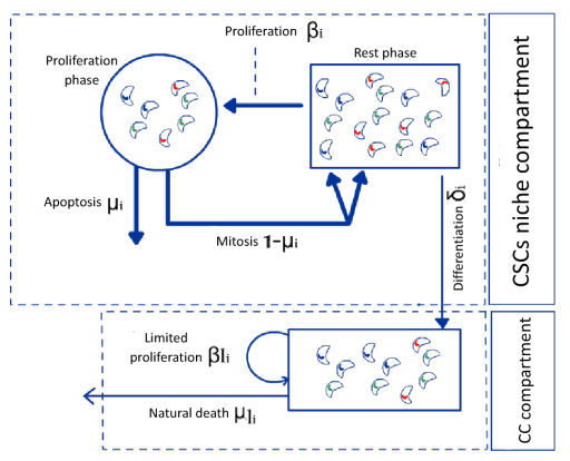
We consider cancer cytotoxic drugs as an optimal control problem to stabilize a heterogeneous tumor by attacking not the most abundant cancer cells, but those that are crucial in the tumor ecosystem. We propose a mathematical cancer stem cell model that translates the hierarchy and heterogeneity of cancer cell types by including highly structured tumorigenic cancer stem cells that yield low differentiated cancer cells. With respect to the optimal control problem, under a certain admissibility hypothesis, the optimal controls of our problem are bang-bang controls. These control treatments can retain the entire tumor in the neighborhood of an equilibrium. We simulate the bang-bang control numerically and demonstrate that the optimal drug scheduling should be administered continuously over long periods with short rest periods. Moreover, our simulations indicate that combining multidrug therapies and monotherapies is more efficient for heterogeneous tumors than using each one separately.
- optimal control theory,
- Pontryagin's maximum principle,
- cancer stem cell,
- cancer dynamics,
- cytotoxic treatment
Citation: Ghassen Haddad, Amira Kebir, Nadia Raissi, Amira Bouhali, Slimane Ben Miled. Optimal control model of tumor treatment in the context of cancer stem cell[J]. Mathematical Biosciences and Engineering, 2022, 19(5): 4627-4642. doi: 10.3934/mbe.2022214

Related Papers:

Abstract

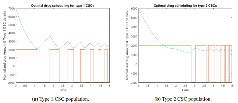
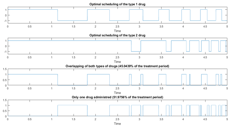
We consider cancer cytotoxic drugs as an optimal control problem to stabilize a heterogeneous tumor by attacking not the most abundant cancer cells, but those that are crucial in the tumor ecosystem. We propose a mathematical cancer stem cell model that translates the hierarchy and heterogeneity of cancer cell types by including highly structured tumorigenic cancer stem cells that yield low differentiated cancer cells. With respect to the optimal control problem, under a certain admissibility hypothesis, the optimal controls of our problem are bang-bang controls. These control treatments can retain the entire tumor in the neighborhood of an equilibrium. We simulate the bang-bang control numerically and demonstrate that the optimal drug scheduling should be administered continuously over long periods with short rest periods. Moreover, our simulations indicate that combining multidrug therapies and monotherapies is more efficient for heterogeneous tumors than using each one separately.

References

[1]	C. E. Eyler, J. N. Rich, Survival of the fittest: cancer stem cells in therapeutic resistance and angiogenesis, J. Clin. Oncol., 26 (2008), 2839. https://doi.org/10.1200/JCO.2007.15.1829 doi: 10.1200/JCO.2007.15.1829
[2]	T. Reya, S. J. Morrison, M. F. Clarke, I. L. Weissman, Stem cells, cancer, and cancer stem cells, Nature, 414 (2001), 105–111. https://doi.org/10.1038/35102167 doi: 10.1038/35102167
[3]	R. Galli, E. Binda, U. Orfanelli, B. Cipelletti, A. Gritti, S. De Vitis, et al., Isolation and characterization of tumorigenic, stem-like neural precursors from human glioblastoma, Cancer Res., 64 (2004), 7011–7021. https://doi.org/10.1158/0008-5472.CAN-04-1364 doi: 10.1158/0008-5472.CAN-04-1364
[4]	T. Kondo, T. Setoguchi, T. Taga, Persistence of a small subpopulation of cancer stem-like cells in the c6 glioma cell line, Proc. Natl. Acad. Sci., 101 (2004), 781–786. https://doi.org/10.1073/pnas.0307618100 doi: 10.1073/pnas.0307618100
[5]	S. K. Singh, C. Hawkins, I. D. Clarke, J. A. Squire, J. Bayani, T. Hide, et al., Identification of human brain tumour initiating cells, Nature, 432 (2004), 396–401. https://doi.org/10.1038/nature03128 doi: 10.1038/nature03128
[6]	J. J. Salk, J. F. Edward, L. A. Loeb, Mutational heterogeneity in human cancers: origin and consequences, Ann. Rev. Pathol. Mech. Dis., 5 (2010), 51–75. https://doi.org/10.1146/annurev-pathol-121808-102113 doi: 10.1146/annurev-pathol-121808-102113
[7]	V. Almendro, A. Marusyk, K. Polyak, Intra-tumour heterogeneity: a looking glass for cancer?, Nat. Rev. Cancer, 12 (2012), 323–334. https://doi.org/10.1038/nrc3261 doi: 10.1038/nrc3261
[8]	P. Dalerba, S. J. Dylla, I. K. Park, R. Liu, X. Wang, R. W. Cho, et al, Phenotypic characterization of human colorectal cancer stem cells, Proc. Natl. Acad. Sci., 104 (2007), 10158–10163. https://doi.org/10.1073/pnas.0703478104 doi: 10.1073/pnas.0703478104
[9]	B. Fang, C. Zheng, L. Liao, Q. Han, Z. Sun, X. Jiang, et al., Identification of human chronic myelogenous leukemia progenitor cells with hemangioblastic characteristics, Blood, 105 (2005), 2733–2740. https://doi.org/10.1182/blood-2004-07-2514 doi: 10.1182/blood-2004-07-2514
[10]	D. Fang, T. K. Nguyen, K. Leishear, R. Finko, A. N. Kulp, S. Hotz, et al., A tumorigenic subpopulation with stem cell properties in melanomas, Cancer Res., 65 (2005), 9328–9337. https://doi.org/10.1158/0008-5472.CAN-05-1343 doi: 10.1158/0008-5472.CAN-05-1343
[11]	T. G. Oliver, R. J. Wechsler-Reya, Getting at the root and stem of brain tumors, Neuron, 42 (2004), 885–888. https://doi.org/10.1016/j.neuron.2004.06.011 doi: 10.1016/j.neuron.2004.06.011
[12]	E. Sagiv, A. Starr, U. Rozovski, R. Khosravi, P. Altevogt, T. Wang, et al., Targeting cd24 for treatment of colorectal and pancreatic cancer by monoclonal antibodies or small interfering RNA, Cancer Res., 68 (2008), 2803–2812. https://doi.org/10.1158/0008-5472.CAN-07-6463 doi: 10.1158/0008-5472.CAN-07-6463
[13]	T. Schatton, N. Y. Frank, M. H. Frank, Identification and targeting of cancer stem cells, Bioessays, 31 (2009), 1038–1049. https://doi.org/10.1002/bies.200900058 doi: 10.1002/bies.200900058
[14]	N. André, L. Padovani, E. Pasquier, Metronomic scheduling of anticancer treatment: the next generation of multitarget therapy?, Future Oncol., 7 (2011), 385–394. https://doi.org/10.2217/fon.11.11 doi: 10.2217/fon.11.11
[15]	D. Hanahan, G. Bergers, E. Bergsland, Less is more, regularly: metronomic dosing of cytotoxic drugs can target tumor angiogenesis in mice, J. Clin. Invest., 105 (2000), 1045–1047. https://doi.org/10.1172/JCI9872 doi: 10.1172/JCI9872
[16]	E. Pasquier, M. Kavallaris, N. André, Metronomic chemotherapy: new rationale for new directions, Nat. Rev. Clin. Oncol., 7 (2010), 455. https://doi.org/10.1038/nrclinonc.2010.82 doi: 10.1038/nrclinonc.2010.82
[17]	J. Lokich, N. Anderson, Dose intensity for bolus versus infusion chemotherapy administration: review of the literature for 27 anti-neoplastic agents, Ann. Oncol., 8 (1997), 15–25. https://doi.org/10.1023/a:1008243806415 doi: 10.1023/a:1008243806415
[18]	D. Sigal, M. Przedborski, D. Sivaloganathan, M. Kohandel, Mathematical modelling of cancer stem cell-targeted immunotherapy, Math. Biosci., 318 (2019), 108269. https://doi.org/10.1016/j.mbs.2019.108269 doi: 10.1016/j.mbs.2019.108269
[19]	S. A. Levin, J. Lei, Q. Nie, Mathematical model of adult stem cell regeneration with cross-talk between genetic and epigenetic regulation, Proc. Natl. Acad. Sci., 111 (2014), E880–E887. https://doi.org/10.1073/pnas.1324267111 doi: 10.1073/pnas.1324267111
[20]	O. Nave, S. Hareli, M. Elbaz, I. H. Iluz, S. Bunimovich-Mendrazitsky, Bcg and il-2 model for bladder cancer treatment with fast and slow dynamics based on spvf method stability analysis, Math. Biosci. Eng., 16 (2019), 5346–5379. https://doi.org/10.3934/mbe.2019267 doi: 10.3934/mbe.2019267
[21]	O. Nave, M. Elbaz, S. Bunimovich-Mendrazitsky, Analysis of a breast cancer mathematical model by a new method to find an optimal protocol for her2-positive cancer, Biosystems, 197 (2020), 104191. https://doi.org/10.1016/j.biosystems.2020.104191 doi: 10.1016/j.biosystems.2020.104191
[22]	D. F. Quail, M. J. Taylor, L. M. Postovit, Microenvironmental regulation of cancer stem cell phenotypes, Curr. Stem Cell Res. Ther., 7 (2012), 593–598. https://doi.org/10.2174/157488812799859838 doi: 10.2174/157488812799859838
[23]	N. H. G. Holford, L. B. Sheiner, Understanding the dose-effect relationship: clinical application of pharmacokinetic-pharmacodynamic models, Clin. Pharmacokinet., 6 (1981), 429–453. https://doi.org/10.2165/00003088-198106060-00002 doi: 10.2165/00003088-198106060-00002
[24]	D. A. Keefe, R. L. Capizzi, S. A. Rudnick, Methotrexate cytotoxicity for L5178Y/Asn-lymphoblasts: relationship of dose and duration of exposure to tumor cell viability, Cancer Res., 42 (1982), 1641–1645.
[25]	W. H. Fleming, R. W. Rishel, Deterministic and Stochastic Optimal Control, Springer Science & Business Media, 2012.
[26]	M. I. Kamien, N. L. Schwartz, Dynamic Optimization : The Calculus of Variations and Optimal Control in Economics and Management, Elsevier, 1998.
[27]	E. Trélat, Contrôle optimal: théorie & applications, Vuibert, 2008.
[28]	L. E. Broder, M. H. Cohen, O. S. Selawry, Treatment of bronchogenic carcinoma: Ii. small cell, Cancer Treat. Rev., 4 (1977), 219–260. https://doi.org/10.1016/s0305-7372(77)80001-7 doi: 10.1016/s0305-7372(77)80001-7
[29]	P. A. Bunn, D. C. Ihde, Small cell bronchogenic carcinoma: a review of therapeutic results, Lung Cancer 1, 1981 (1981), 169–208. https://doi.org/10.1007/978-94-009-8207-9_8 doi: 10.1007/978-94-009-8207-9_8
[30]	K. Staňková, J. S. Brown, W. S. Dalton, R. A. Gatenby, Optimizing cancer treatment using game theory: a review, JAMA Oncol., 5 (2018), 96–103. https://doi.org/10.1001/jamaoncol.2018.3395 doi: 10.1001/jamaoncol.2018.3395
[31]	G. Bonadonna, M. Zambetti, P. Valagussa, Sequential or alternating doxorubicin and cmf regimens in breast cancer with more than three positive nodes: ten-year results, Jama, 273 (1995), 542–547. https://doi.org/10.1001/jama.1995.03520310040027 doi: 10.1001/jama.1995.03520310040027
[32]	P. Alberto, K. W. Brunner, G. Martz, J. Obrecht, R. W. Sonntag, Treatment of bronchogenic carcinoma with simultaneous or sequential combination chemotherapy, including methotrexate, cyclophosphamide, procarbazine and vincristine, Cancer, 38 (1976), 2208–2216. https://doi.org/10.1002/1097-0142(197612)38:6<2208::AID-CNCR2820380603>3.0.CO; 2-H
[33]	G. Dontu, K. W. Jackson, E. McNicholas, M. J. Kawamura, W. M. Abdallah, M. S. Wicha, Role of notch signaling in cell-fate determination of human mammary stem/progenitor cells, Breast Cancer Res., 6 (2004), R605. https://doi.org/10.1186/bcr920 doi: 10.1186/bcr920
[34]	S. S. Kanwar, Y. Yu, J. Nautiyal, B. B. Patel, A. P. N. Majumdar, The wnt/$\beta$-catenin pathway regulates growth and maintenance of colonospheres, Mol. Cancer, 9 (2010), 212. https://doi.org/10.1186/1476-4598-9-212 doi: 10.1186/1476-4598-9-212
[35]	A. Shiras, S. T. Chettiar, V. Shepal, G. Rajendran, G. R. Prasad, P. Shastry, Spontaneous transformation of human adult nontumorigenic stem cells to cancer stem cells is driven by genomic instability in a human model of glioblastoma, Stem Cells, 25 (2007), 1478–1489. https://doi.org/10.1186/1476-4598-9-212 doi: 10.1186/1476-4598-9-212
[36]	I. V. Ulasov, S. Nandi, M. Dey, A. M. Sonabend, M. S. Lesniak, Inhibition of sonic hedgehog and notch pathways enhances sensitivity of cd133+ glioma stem cells to temozolomide therapy, Mol. Med., 17 (2011), 103–112. https://doi.org/10.2119/molmed.2010.00062 doi: 10.2119/molmed.2010.00062
[37]	N. Sanai, A. Alvarez-Buylla, M. S. Berger, Neural stem cells and the origin of gliomas, N. Engl. J. Med., 353 (2005), 811–822. https://doi.org/10.1056/NEJMra043666 doi: 10.1056/NEJMra043666

Reader Comments

Your name:*

Email:*
© 2022 the Author(s), licensee AIMS Press. This is an open access article distributed under the terms of the Creative Commons Attribution License (http://creativecommons.org/licenses/by/4.0)