An optimal control model to design strategies for reducing the spread of the Ebola virus disease

Rama Seck; Diène Ngom; Benjamin Ivorra; Ángel M. Ramos; Rama Seck; Diène Ngom; Benjamin Ivorra; Ángel M. Ramos

doi:10.3934/mbe.2022082

Mathematical Biosciences and Engineering

2022, Volume 19, Issue 2: 1746-1774. doi: 10.3934/mbe.2022082

Previous Article Next Article

Research article Special Issues

An optimal control model to design strategies for reducing the spread of the Ebola virus disease

1.
Laboratory of Numerical Analysis and Computer Science, Applied Mathematics Section, Gaston Berger University, Saint-Louis, 209-IRD & UMMISCO-UGB, Senegal
2.
Mathematics and Applications Laboratory, Mathematics Department, Assane Seck University, Bp: 523, Ziguinchor, 209-IRD & UMMISCO-UGB, Senegal
3.
Interdisciplinary Mathematics Institute, Department of Applied Mathematics and Mathematical Analysis, Complutense University of Madrid, Plaza de Ciencias, 3, 28040 Madrid, Spain

Academic Editor: Masaki Ogura

Received: 20 August 2021 Accepted: 22 November 2021 Published: 16 December 2021

In this work, we formulate an epidemiological model for studying the spread of Ebola virus disease in a considered territory. This model includes the effect of various control measures, such as: vaccination, education campaigns, early detection campaigns, increase of sanitary measures in hospital, quarantine of infected individuals and restriction of movement between geographical areas. Using optimal control theory, we determine an optimal control strategy which aims to reduce the number of infected individuals, according to some operative restrictions (e.g., economical, logistic, etc.). Furthermore, we study the existence and uniqueness of the optimal control. Finally, we illustrate the interest of the obtained results by considering numerical experiments based on real data.
- epidemiological modeling,
- optimal control,
- Ebola virus disease,
- deterministic models
Citation: Rama Seck, Diène Ngom, Benjamin Ivorra, Ángel M. Ramos. An optimal control model to design strategies for reducing the spread of the Ebola virus disease[J]. Mathematical Biosciences and Engineering, 2022, 19(2): 1746-1774. doi: 10.3934/mbe.2022082

Related Papers:

Abstract

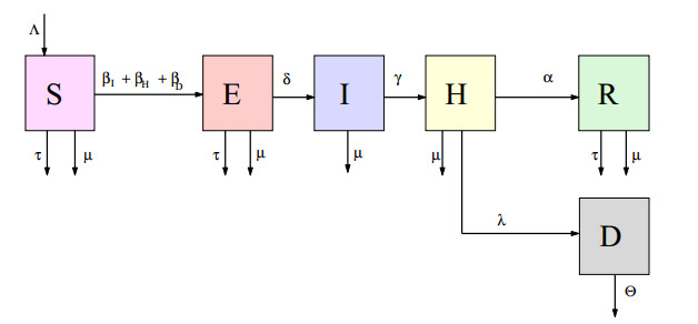
In this work, we formulate an epidemiological model for studying the spread of Ebola virus disease in a considered territory. This model includes the effect of various control measures, such as: vaccination, education campaigns, early detection campaigns, increase of sanitary measures in hospital, quarantine of infected individuals and restriction of movement between geographical areas. Using optimal control theory, we determine an optimal control strategy which aims to reduce the number of infected individuals, according to some operative restrictions (e.g., economical, logistic, etc.). Furthermore, we study the existence and uniqueness of the optimal control. Finally, we illustrate the interest of the obtained results by considering numerical experiments based on real data.

References

[1]	M. Anderson, R. M. May, Population Biology of Infectious Diseases: Part 1, Princeton University Press, (1979), 361–367. doi: 10.1038/280361a0.
[2]	B. Ivorra, M. R. Ferrández, M. Vela-Pérez, A. M. Ramos, Mathematical modeling of the spread of the coronavirus disease 2019 (COVID-19) taking into account the undetected infections. The case of China, Commun. Nonlinear Sci. Numer. Simul., 88 (2020), 105303, doi: 10.1016/j.cnsns.2020.105303, 2020. doi: 10.1016/j.cnsns.2020.105303
[3]	B. Ivorra, D. Ngom, A. M. Ramos, Be-codis: a mathematical model to predict the risk of human diseases spread between countries–-validation and application to the 2014–2015 ebola virus disease epidemic, Bull. Math. Biol., 77 (2015), 1668–1704. doi: 10.1007/s11538-015-0100-x. doi: 10.1007/s11538-015-0100-x
[4]	A. M. Ramos, M. Vela-Pérez, M. R. Ferrández, A. B.Kubik, B. Ivorra, A simple but complex enough $\theta$-SIR type model to be used with COVID-19 real data. Application to the case of Italy, Phys. D Nonlinear Phenom., 421 (2021), 132839. doi: 10.1016/j.physd.2020.132839. doi: 10.1016/j.physd.2020.132839
[5]	A. M. Ramos, M. Vela-Pérez, M. R. Ferrández, A. B. Kubik, B. Ivorra, Modeling the impact of SARS-CoV-2 variants and vaccines on the spread of COVID-19, Commun. Nonlinear Sci. Numer. Simul., 2021 (2021). doi: 10.13140/RG.2.2.32580.24967/2. doi: 10.13140/RG.2.2.32580.24967/2
[6]	I. Area, J. Losada, F. Ndairou, J. J. Nieto, D. D. Tcheutia, Mathematical modeling of 2014 Ebola outbreak, Math. Methods Appl. Sci., 40 (2017), 6114–6122. doi: 10.1002/mma.3794. doi: 10.1002/mma.3794
[7]	S. D. D. Njankou, F. Nyabadza, An optimal control model for Ebola virus disease, J. Biol. Syst., 24 (2016), 29–49. doi: 10.1142/S0218339016500029. doi: 10.1142/S0218339016500029
[8]	A. Rachah, D. F. M. Torres, Mathematical modelling, simulation, and optimal control of the 2014 Ebola outbreak in West Africa, Discrete Dyn. Nat. Soc., 2015 (2015). doi: 10.1155/2015/842792. doi: 10.1155/2015/842792
[9]	B. Ivorra, B. Martínez-López, J. M. Sánchez-Vizcaíno, A. M. Ramos, Mathematical formulation and validation of the Be-FAST model for classical swine fever virus spread between and within farms, Ann. Oper. Res., 219 (2014), 25–47. doi: 10.1007/s10479-012-1257-4. doi: 10.1007/s10479-012-1257-4
[10]	B. Martínez-López, B. Ivorra, A. M. Ramos, J. M. Sánchez-Vizcaíno, A novel spatial and stochastic model to evaluate the within- and between-farm transmission of classical swine fever virus. Ⅰ. General concepts and description of the model, Vet. Microbiol., 147 (2011), 300–309. doi: 10.1016/j.vetmic.2010.07.009. doi: 10.1016/j.vetmic.2010.07.009
[11]	H. R. Thieme, Mathematics in Population Biology, Princeton University Press, 2003. doi: 10.1515/9780691187655.
[12]	T. T. Yusuf, F. Benyah, Optimal control of vaccination and treatment for an SIR epidemiological model, World J. Modell. Simul., 8 (2012), 194–204.
[13]	A. A. Lashari, G. Zaman, Optimal control of a vertor-borne disease with horizontal transmission, Nonlinear Anal. Real World Appl., 13 (2012), 203–212. doi: 10.1016/j.nonrwa.2011.07.026. doi: 10.1016/j.nonrwa.2011.07.026
[14]	R. T. D Emond, B. Evans, E. T. W Bowen, G. Lloyd, A case of ebola virus infection, Br. Med. J., 2 (1977), 541–544. doi: 10.1136/bmj.2.6086.541. doi: 10.1136/bmj.2.6086.541
[15]	C. J. Peters, J. W. Peters, An introduction to ebola: The virus and the disease, J. Infect. Dis., 179 (1999). doi: 10.1086/514322. doi: 10.1086/514322
[16]	WHO, Global alert and response: Ebola virus disease, 2016. Available from: https://www.who.int/health-topics/ebola
[17]	B. Ivorra, D. Ngom, A. M. Ramos, Stability and sensitivity analysis of be-codis: an epidemiological model to predict the spread of human diseases between countries—validation with data from the 2014–16 west african ebola virus disease epidemic, Electron. J. Differ. Equations, 62 (2020), 1–29.
[18]	D. N. Edith, G. C. E. Mbah, B. E. Bassey, Optimal control analysis model of Ebola virus infection: impact of socio-economic status, Int. J. Appl. Sci. Math., 6 (2020), 2394–2894.
[19]	F. Clarke, Functional Analysis, Calculus of Variations and Optimal Control. Springer London, 2013. doi: 10.1007/978-1-4471-4820-3.
[20]	J. Legrand, R. F. Grais, P. Y. Boelle, A. J. Valleron, A. Flahault, Understanding the dynamics of ebola epidemics, Med. Hypotheses., 135 (2007), 610–621. doi: 10.1017/S0950268806007217. doi: 10.1017/S0950268806007217
[21]	M. I. Meltzer, C. Y. Atkins, S. Santibanez, B. Knust, B. W. Petersen, E. D. Ervin, et al., Estimating the future number of cases in the ebola epidemic - Liberia and Sierra Leone, 2014–2015, MMWR, 63 (2014).
[22]	WHO Response Team, Ebola virus disease in west africa - the first 9 months of the epidemic and forward projections, N. Engl. J. Med., 371 (2014), 1481–1495. doi: 10.1056/NEJMoa1411100. doi: 10.1056/NEJMoa1411100
[23]	D. Fisman, E. Khoo, A. Tuite, Early epidemic dynamics of the west african 2014 ebola outbreak: estimates derived with a simple two-parameter model, PLOS Curr., 2014 (2014). doi: 10.1371/currents.outbreaks.89c0d3783f36958d96ebbae97348d5710. doi: 10.1371/currents.outbreaks.89c0d3783f36958d96ebbae97348d5710
[24]	N. Hernandez-Ceron, Z. Feng, C. Castillo-Chavez, Discrete epidemic models with arbitrary stage distributions and applications to disease control, Bull. Math. Biol., 75 (2013), 1716–1746. doi: 10.1007/s11538-013-9866-x. doi: 10.1007/s11538-013-9866-x
[25]	G. Giordano, F. Blanchini, R. Bruno, P. Colaneri, A. Di Filippo, A. Di Matteo, et al., Modelling the covid-19 epidemic and implementation of population-wide interventions in Italy, Nat. Med., 26 (2020), 855–860. doi: 10.1038/s41591-020-0883-7. doi: 10.1038/s41591-020-0883-7
[26]	M. Barro, A. Guiro, D. Ouedraogo, Optimal control of a SIR epidemic model with general incidence function and a time delays, CUBO, 20 (2018), 53–66. doi: 10.4067/S0719-06462018000200053. doi: 10.4067/S0719-06462018000200053
[27]	E. B. M. Bashier, K. C. Patidar, Optimal control of an epidemiological model with multiple time delays, Appl. Math. Comput., 292 (2017), 47–56. doi: 10.1016/j.amc.2016.07.009. doi: 10.1016/j.amc.2016.07.009
[28]	S. Nanda, H. Moore, S. Lenhart, Optimal control of treatment in a mathematical model of chronic myelogenous leukemia, Math. Biosci., 210 (2007), 143–156. doi: 10.1016/j.mbs.2007.05.003. doi: 10.1016/j.mbs.2007.05.003
[29]	L. S. Pontryagin, V. G. Boltyanskii, R. V. Gamkrelidze, E. F. Mishchenko, The Mathematical Theory of Optimal Processes, CRC Press, 1987.
[30]	M. Tahir, G. Zaman, S. I. A. Shah, Evaluation and control estimation strategy for three acting play diseases with six control variables, Cogent Math. Stat., 7 (2020), 1805871. doi: 10.1057/jors.1965.92. doi: 10.1057/jors.1965.92
[31]	I. Area, F. Ndairou, J. J Nietto, C. J. Silva, D. F. M. Torres, Ebola model and optimal control with vaccination constraints, J. Ind. Manag. Optim., 14 (2018), 427–446. doi: 10.3934/jimo.2017054. doi: 10.3934/jimo.2017054
[32]	S. Lenhart, J. T. Workman, Optimal Control Applied to Biological Models, in: Mathematical And Computational Biology Series. Chapman & Hall/CRC, London, UK, 2007. doi: 10.1201/9781420011418.

Reader Comments

Your name:*

Email:*
© 2022 the Author(s), licensee AIMS Press. This is an open access article distributed under the terms of the Creative Commons Attribution License (http://creativecommons.org/licenses/by/4.0)