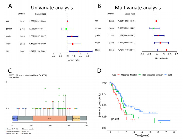
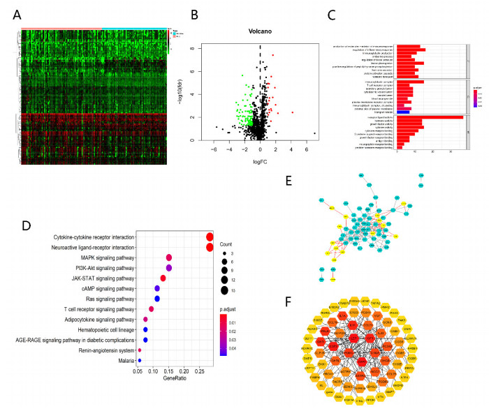
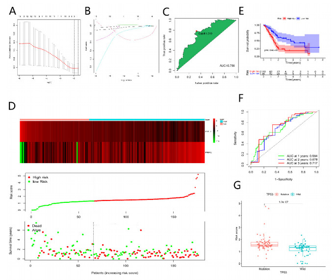
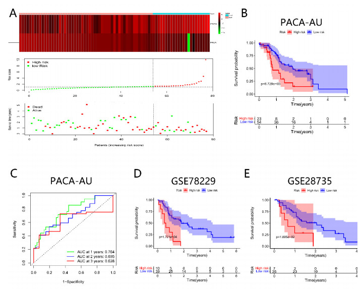
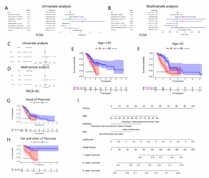
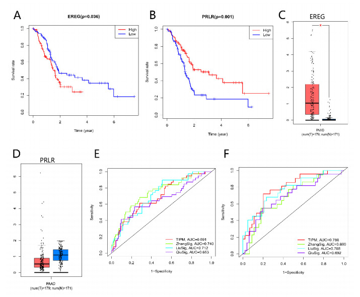
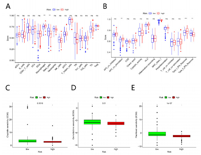
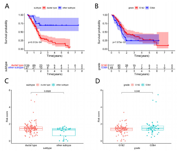
Pancreatic cancer (PC) is a highly fatal disease correlated with an inferior prognosis. The tumor protein p53 (TP53) is one of the frequent mutant genes in PC and has been implicated in prognosis. We collected somatic mutation data, RNA sequencing data, and clinical information of PC samples in the Cancer Genome Atlas (TCGA) database. TP53 mutation was an independent prognostic predictor of PC patients. According to TP53 status, Gene set enrichment analysis (GSEA) suggested that TP53 mutations were related to the immunophenotype of pancreatic cancer. We identified 102 differentially expressed immune genes (DEIGs) based on TP53 mutation status and developed a TP53-associated immune prognostic model (TIPM), including Epiregulin (EREG) and Prolactin receptor (PRLR). TIPM identified the high-risk group with poor outcomes and more significant response potential to cisplatin, gemcitabine, and paclitaxel therapies. And we verified the TIPM in the International Cancer Genome Consortium (ICGC) cohort (PACA-AU) and Gene Expression Omnibus (GEO) cohort (GSE78229 and GSE28735). Finally, we developed a nomogram that reliably predicts overall survival in PC patients on the bias of TIPM and other clinicopathological factors. Our study indicates that the TIPM derived from TP53 mutation patterns might be an underlying prognostic therapeutic target. But more comprehensive researches with a large sample size is necessary to confirm the potential.
Citation: Yi Liu, Long Cheng, Xiangyang Song, Chao Li, Jiantao Zhang, Lei Wang. A TP53-associated immune prognostic signature for the prediction of the overall survival and therapeutic responses in pancreatic cancer[J]. Mathematical Biosciences and Engineering, 2022, 19(1): 191-208. doi: 10.3934/mbe.2022010
Pancreatic cancer (PC) is a highly fatal disease correlated with an inferior prognosis. The tumor protein p53 (TP53) is one of the frequent mutant genes in PC and has been implicated in prognosis. We collected somatic mutation data, RNA sequencing data, and clinical information of PC samples in the Cancer Genome Atlas (TCGA) database. TP53 mutation was an independent prognostic predictor of PC patients. According to TP53 status, Gene set enrichment analysis (GSEA) suggested that TP53 mutations were related to the immunophenotype of pancreatic cancer. We identified 102 differentially expressed immune genes (DEIGs) based on TP53 mutation status and developed a TP53-associated immune prognostic model (TIPM), including Epiregulin (EREG) and Prolactin receptor (PRLR). TIPM identified the high-risk group with poor outcomes and more significant response potential to cisplatin, gemcitabine, and paclitaxel therapies. And we verified the TIPM in the International Cancer Genome Consortium (ICGC) cohort (PACA-AU) and Gene Expression Omnibus (GEO) cohort (GSE78229 and GSE28735). Finally, we developed a nomogram that reliably predicts overall survival in PC patients on the bias of TIPM and other clinicopathological factors. Our study indicates that the TIPM derived from TP53 mutation patterns might be an underlying prognostic therapeutic target. But more comprehensive researches with a large sample size is necessary to confirm the potential.

| [1] | M. Ilic, I. Ilic, Epidemiology of pancreatic cancer, World J. Gastroenterol., 22 (2016), 9694-9705. doi: 10.3748/wjg.v22.i44.9694. |
| [2] | J. D. Mizrahi, R. Surana, J. W. Valle, R. T. Shroff, Pancreatic cancer, Lancet, 395 (2020), 2008-2020. doi: 10.1016/S0140-6736(20)30974-0. |
| [3] | T. Kamisawa, L. D. Wood, T. Itoi, K. Takaori, Pancreatic cancer, Lancet, 388 (2016), 73-85. doi: 10.1016/S0140-6736(16)00141-0. |
| [4] |
A. D. Singhi, E. J. Koay, S. T. Chari, A. Maitra, Early detection of pancreatic cancer: opportunities and challenges, Gastroenterology, 156 (2019), 2024-2040. doi: 10.1053/j.gastro.2019.01.259. doi: 10.1053/j.gastro.2019.01.259

|
| [5] | B. Zhang, Q. Wu, B. Li, D. Wang, L. Wang, Y. L. Zhou, mA regulator-mediated methylation modification patterns and tumor microenvironment infiltration characterization in gastric cancer, Mol. Cancer, 19 (2020), 53. doi: 10.1186/s12943-020-01170-0. |
| [6] | Y. Ino, R. Yamazaki-Itoh, K. Shimada, M. Iwasaki, T. Kosuge, Y. Kanai, et al., Immune cell infiltration as an indicator of the immune microenvironment of pancreatic cancer, Br. J. Cancer, 108 (2013), 914-923. doi: 10.1038/bjc.2013.32. |
| [7] |
W. J. Ho, E. M. Jaffee, L. Zheng, The tumour microenvironment in pancreatic cancer-clinical challenges and opportunities, Nat. Rev. Clin. Oncol., 17 (2020), 527-540. doi: 10.1038/s41571-020-0363-5. doi: 10.1038/s41571-020-0363-5
|
| [8] | A. O. Giacomelli, X. Yang, R. E. Lintner, J. M. McFarland, M. Duby, J. Kim, et al., Mutational processes shape the landscape of TP53 mutations in human cancer, Nat. Genet., 50 (2018), 1381-1387. doi: 10.1038/s41588-018-0204-y. |
| [9] |
A. J. Levine, M. Oren, The first 30 years of p53: growing ever more complex, Nat. Rev. Cancer, 9 (2009), 749-758. doi: 10.1038/nrc2723. doi: 10.1038/nrc2723
|
| [10] |
R. Brosh, V. Rotter, When mutants gain new powers: news from the mutant p53 field, Nat. Rev. Cancer, 9 (2009), 701-713. doi: 10.1038/nrc2693. doi: 10.1038/nrc2693
|
| [11] | S. P. Dowell, P. O. Wilson, N. W. Derias, D. P. Lane, P. A. Hall, Clinical utility of the immunocytochemical detection of p53 protein in cytological specimens, Cancer Res., 54 (1994), 2914-2918. |
| [12] |
I. Ringshausen, C. C. O'Shea, A. J. Finch, L. B. Swigart, G. I. Evan, Mdm2 is critically and continuously required to suppress lethal p53 activity in vivo, Cancer Cell, 10 (2006), 501-514. doi: 10.3748/10.1016/j.ccr.2006.10.010. doi: 10.3748/10.1016/j.ccr.2006.10.010
|
| [13] | V. J. N. Bykov, S. E. Eriksson, J. Bianchi, K. G. Wiman, Targeting mutant p53 for efficient cancer therapy, Nat. Rev. Cancer, 18 (2018). doi: 10.1038/nrc.2017.109. |
| [14] | X. Liu, B. Chen, J. Chen, S. Sun, A novel tp53-associated nomogram to predict the overall survival in patients with pancreatic cancer, BMC Cancer, 21 (2021), 335. doi: 10.1186/s12885-021-08066-2. |
| [15] | F. Zhang, W. Zhong, H. Li, K. Huang, M. Yu, Y. Liu, TP53 mutational status-based genomic signature for prognosis and predicting therapeutic response in pancreatic cancer, Front. Cell. Dev. Biol., 9 (2021), 665265. doi: 10.3389/fcell.2021.665265. |
| [16] | H. Sun, B. Zhang, H. Li, The roles of frequently mutated genes of pancreatic cancer in regulation of tumor microenvironment, Technol. Cancer Res. Treat., 19 (2020), 1533033820920969. doi: 10.1177/1533033820920969. |
| [17] | S. Hashimoto, S. Furukawa, A. Hashimoto, A. Tsutaho, A. Fukao, Y. Sakamura, et al., ARF6 and AMAP1 are major targets of and mutations to promote invasion, PD-L1 dynamics, and immune evasion of pancreatic cancer, Proc. Nat. Acad. Sci. U. S. A., 116 (2019), 17450-17459. doi: 10.1073/pnas.1901765116. |
| [18] | D. Toro-Domínguez, J. Martorell-Marugán, R. López-Domínguez, A. García-Moreno, V. González-Rumayor, M. E. Alarcón-Riquelme, et al., ImaGEO: integrative gene expression meta-analysis from GEO database, Bioinformatics, 35 (2019), 880-882. doi: 10.1093/bioinformatics/bty721. |
| [19] | A. Subramanian, P. Tamayo, V. K. Mootha, S. Mukherjee, B. L. Ebert, M. A. Gillette, et al., Gene set enrichment analysis: a knowledge-based approach for interpreting genome-wide expression profiles, Proc. Nat. Acad. Sci. U. S. A., 102 (2005), 15545-15550. doi: 10.1073/pnas.0506580102. |
| [20] | S. Bhattacharya, S. Andorf, L. Gomes, P. Dunn, H. Schaefer, J. Pontius, et al., ImmPort: disseminating data to the public for the future of immunology, Immunol. Res., 58 (2014), 234-239. doi: 10.1007/s12026-014-8516-1. |
| [21] | D. Szklarczyk, A. Franceschini, S. Wyder, K. Forslund, D. Heller, J. Huerta-Cepas, et al., STRING v10: protein-protein interaction networks, integrated over the tree of life, Nucleic Acids Res., 43 (2015), D447-D452. doi: 10.1093/nar/gku1003. |
| [22] | P. Shannon, A. Markiel, O. Ozier, N. S. Baliga, J. T. Wang, D. Ramage, et al., Cytoscape: a software environment for integrated models of biomolecular interaction networks, Genome Res., 13 (2003), 2498-2504. doi: 10.1101/gr.1239303. |
| [23] | G. D. Bader, C. W. V. Hogue, An automated method for finding molecular complexes in large protein interaction networks, BMC Bioinf., 4 (2003), 2. doi: 10.1186/1471-2105-4-2. |
| [24] | Y. Zhou, B. Zhou, L. Pache, M. Chang, A. H. Khodabakhshi, O. Tanaseichuk, et al., Metascape provides a biologist-oriented resource for the analysis of systems-level datasets, Nat. Commun., 10 (2019), 1523. doi: 10.1038/s41467-019-09234-6. |
| [25] | Z. Tang, C. Li, B. Kang, G. Gao, C. Li, Z. Zhang, GEPIA: a web server for cancer and normal gene expression profiling and interactive analyses, Nucleic Acids Res., 45 (2017). doi: 10.1093/nar/gkx247. |
| [26] | A. Subramanian, P. Tamayo, V. K. Mootha, S. Mukherjee, B. L. Ebert, M. A. Gillette, et al., Gene set enrichment analysis: a knowledge-based approach for interpreting genome-wide expression profiles, Proc. Nat. Acad. Sci. U. S. A., 102 (2005), 15545-15550. doi: 10.1073/pnas.0506580102. |
| [27] | W. Yang, J. Soares, P. Greninger, E. J. Edelman, H. Lightfoot, S. Forbes, et al., Genomics of Drug Sensitivity in Cancer (GDSC): a resource for therapeutic biomarker discovery in cancer cells, Nucleic Acids Res., 41 (2013), D955-D961. doi: 10.1093/nar/gks1111. |
| [28] | P. Geeleher, N. J. Cox, R. S. Huang, Clinical drug response can be predicted using baseline gene expression levels and in vitro drug sensitivity in cell lines, Genome Biol., 15 (2014), R47. doi: 10.1186/gb-2014-15-3-r47. |
| [29] | C. J. Qiu, X. B. Wang, Z. R. Zheng, C. Z. Yang, K. Lin, K. Zhang, et al., Development and validation of a ferroptosis-related prognostic model in pancreatic cancer, Invest. New Drugs, 2021. doi: 10.1007/s10637-021-01114-5. |
| [30] | M. Miyazawa, M. Katsuda, M. Kawai, S. Hirono, K. I. Okada, Y. Kitahata, et al., Advances in immunotherapy for pancreatic ductal adenocarcinoma, J. Hepato-Biliary-Pancreat. Sci., 28 (2021), 419-430. doi: 10.1002/jhbp.944. |
| [31] | F. Skoulidis, M. E. Goldberg, D. M. Greenawalt, M. D. Hellmann, M. M. Awad, J. F. Gainor, et al., STK11/LKB1 mutations and PD-1 inhibitor resistance in KRAS-mutant lung adenocarcinoma, Cancer Discov., 8 (2018), 822-835. doi: 10.1158/2159-8290.CD-18-0099. |
| [32] | Z. Y. Dong, W. Z. Zhong, X. C. Zhang, J. Su, Z. Xie, S. Y. Liu, et al., Potential predictive value of and mutation status for response to PD-1 blockade immunotherapy in lung adenocarcinoma, Clin. Cancer Res., 23 (2017), 3012-3024. doi: 10.1158/1078-0432.CCR-16-2554. |
| [33] | A. K. Witkiewicz, E. A. McMillan, U. Balaji, G. Baek, W. C. Lin, J. Mansour, et al., Whole-exome sequencing of pancreatic cancer defines genetic diversity and therapeutic targets, Nat. Commun., 6 (2015), 6744. doi: 10.1038/ncomms7744. |
| [34] | Z. Zhu, J. Kleeff, H. Friess, L. Wang, A. Zimmermann, Y. Yarden, et al., Epiregulin is up-regulated in pancreatic cancer and stimulates pancreatic cancer cell growth, Biochem. Biophys. Res. Commun., 273 (2000), 1019-1024. doi: 10.1006/bbrc.2000.3033. |
| [35] |
D. J. Riese, R. L. Cullum, Epiregulin: roles in normal physiology and cancer, Semin. Cell Dev. Biol., 28 (2014), 49-56. doi: 10.1016/j.semcdb.2014.03.005. doi: 10.1016/j.semcdb.2014.03.005
|
| [36] | F. Bormann, S. Stinzing, S. Tierling, M. Morkel, M. R. Markelova, J. Walter, et al., Epigenetic regulation of amphiregulin and epiregulin in colorectal cancer, Int. J. Cancer, 144 (2019), 569-581. doi: 10.1002/ijc.31892. |
| [37] | J. Zhang, K. Iwanaga, K. C. Choi, M. Wislez, M. G. Raso, W. Wei, et al., Intratumoral epiregulin is a marker of advanced disease in non-small cell lung cancer patients and confers invasive properties on EGFR-mutant cells, Cancer Prev. Res. (Phila), 1 (2008), 201-207. doi: 10.1158/1940-6207.CAPR-08-0014. |
| [38] |
R. S. Herbst, Review of epidermal growth factor receptor biology, Int. J. Radiat. Oncol. Biol. Phys., 59 (2004), 21-26. doi: 10.1016/j.ijrobp.2003.11.041. doi: 10.1016/j.ijrobp.2003.11.041
|
| [39] |
C. M. Sloss, F. Wang, M. A. Palladino, J. C. Cusack, Activation of EGFR by proteasome inhibition requires HB-EGF in pancreatic cancer cells, Oncogene, 29 (2010), 3146-3152. doi: 10.1038/onc.2010.52. doi: 10.1038/onc.2010.52
|
| [40] |
V. Bernard, J. Young, P. Chanson, N. Binart, New insights in prolactin: pathological implications, Nat. Rev. Endocrinol., 11 (2015), 265-275. doi: 10.1038/nrendo.2015.36. doi: 10.1038/nrendo.2015.36
|
| [41] | P. Dandawate, G. Kaushik, C. Ghosh, D. Standing, A. A. Ali Sayed, S. Choudhury, et al., Diphenylbutylpiperidine antipsychotic drugs inhibit prolactin receptor signaling to reduce growth of pancreatic ductal adenocarcinoma in mice, Gastroenterology, 158 (2020). doi: 10.1053/j.gastro.2019.11.279. |
| [42] | M. Tandon, G. M. Coudriet, A. Criscimanna, M. Socorro, M. Eliliwi, A. D. Singhi, et al., Prolactin promotes fibrosis and pancreatic cancer progression, Cancer Res., 79 (2019), 5316-5327. doi: 10.1158/0008-5472.CAN-18-3064. |
| [43] | H. Nie, P. Q. Huang, S. H. Jiang, Q. Yang, L. P. Hu, X. M. Yang, et al., The short isoform of PRLR suppresses the pentose phosphate pathway and nucleotide synthesis through the NEK9-Hippo axis in pancreatic cancer, Theranostics, 11 (2021), 3898-3915. doi: 10.7150/thno.51712. |
| [44] |
J. Yang, Y. Li, Z. Sun, H. Zhan, Macrophages in pancreatic cancer: An immunometabolic perspective, Cancer Lett., 498 (2021), 188-200. doi: 10.1016/j.canlet.2020.10.029. doi: 10.1016/j.canlet.2020.10.029
|
| [45] | S. S. Linton, T. Abraham, J. Liao, G. A. Clawson, P. J. Butler, T. Fox, et al., Tumor-promoting effects of pancreatic cancer cell exosomes on THP-1-derived macrophages, PLoS One, 13 (2018), e0206759. doi: 10.1371/journal.pone.0206759. |
 mbe-19-01-010-Supplementary.pdf mbe-19-01-010-Supplementary.pdf |
 |
Figures(8)

Yi Liu, Long Cheng, Xiangyang Song, Chao Li, Jiantao Zhang, Lei Wang. A TP53-associated immune prognostic signature for the prediction of the overall survival and therapeutic responses in pancreatic cancer[J]. Mathematical Biosciences and Engineering, 2022, 19(1): 191-208. doi: 10.3934/mbe.2022010


 DownLoad: