Virtual experimentation is a widely used approach for predicting systems behaviour especially in situations where resources for physical experiments are very limited. For example, targeted treatment inside the human body is particularly challenging, and as such, modeling and simulation is utilised to aid planning before a specific treatment is administered. In such approaches, precise treatment, as it is the case in radiotherapy, is used to administer a maximum dose to the infected regions while minimizing the effect on normal tissue. Complicated cancers such as leukemia present even greater challenges due to their presentation in liquid form and not being localised in one area. As such, science has led to the development of targeted drug delivery, where the infected cells can be specifically targeted anywhere in the body.
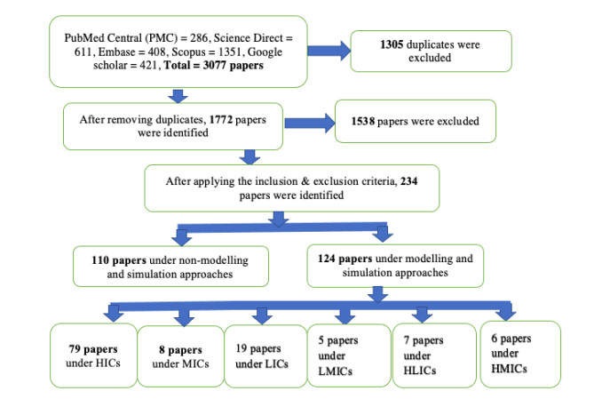
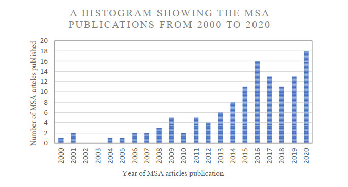
Despite the great prospects and advances of these modeling and simulation tools in the design and delivery of targeted drugs, their use by Low and Middle Income Countries (LMICs) researchers and clinicians is still very limited. This paper therefore reviews the modeling and simulation approaches for leukemia treatment using nanoparticles as an example for virtual experimentation. A systematic review from various databases was carried out for studies that involved cancer treatment approaches through modeling and simulation with emphasis to data collected from LMICs. Results indicated that whereas there is an increasing trend in the use of modeling and simulation approaches, their uptake in LMICs is still limited. According to the review data collected, there is a clear need to employ these tools as key approaches for the planning of targeted drug treatment approaches.
Citation: Henry Fenekansi Kiwumulo, Haruna Muwonge, Charles Ibingira, John Baptist Kirabira, Robert Tamale. Ssekitoleko. A systematic review of modeling and simulation approaches in designing targeted treatment technologies for Leukemia Cancer in low and middle income countries[J]. Mathematical Biosciences and Engineering, 2021, 18(6): 8149-8173. doi: 10.3934/mbe.2021404
Virtual experimentation is a widely used approach for predicting systems behaviour especially in situations where resources for physical experiments are very limited. For example, targeted treatment inside the human body is particularly challenging, and as such, modeling and simulation is utilised to aid planning before a specific treatment is administered. In such approaches, precise treatment, as it is the case in radiotherapy, is used to administer a maximum dose to the infected regions while minimizing the effect on normal tissue. Complicated cancers such as leukemia present even greater challenges due to their presentation in liquid form and not being localised in one area. As such, science has led to the development of targeted drug delivery, where the infected cells can be specifically targeted anywhere in the body.
Despite the great prospects and advances of these modeling and simulation tools in the design and delivery of targeted drugs, their use by Low and Middle Income Countries (LMICs) researchers and clinicians is still very limited. This paper therefore reviews the modeling and simulation approaches for leukemia treatment using nanoparticles as an example for virtual experimentation. A systematic review from various databases was carried out for studies that involved cancer treatment approaches through modeling and simulation with emphasis to data collected from LMICs. Results indicated that whereas there is an increasing trend in the use of modeling and simulation approaches, their uptake in LMICs is still limited. According to the review data collected, there is a clear need to employ these tools as key approaches for the planning of targeted drug treatment approaches.

| [1] |
H. Sharma, P. K. Mishra, S. Talegaonkar, B. Vaidya, Metal nanoparticles: a theranostic nanotool against cancer, Drug Discov. Today, 20 (2015), 1143-1151. doi: 10.1016/j.drudis.2015.05.009

|
| [2] | O. Ramirez, P. Aristizabal, A. Zaidi, R. C. Ribeiro, L. E. Bravo, Implementing a Childhood Cancer Outcomes Surveillance System Within a Population-Based Cancer Registry, J. Global Oncology., (2018), 1-11. |
| [3] | J. S. Slone, A. K. Slone, O. Wally, P. Semetsa, M. Raletshegwana, S. Alisanski, et al., Establishing a Pediatric Hematology-Oncology Program in Botswana, J. Glob. Oncol., (2018), 1-9. |
| [4] | R. L. Siegel, K. D. Miller, A. Jemal, Cancer statistics, 2016, CA: Cancer J. Clin., 66 (2016), 7-30. |
| [5] | E. Jabbour, H. Kantarjian, Chronic myeloid leukemia: 2012 update on diagnosis, monitoring, and management, Am. J. Hematol., 87 (2012), 1037-1045. |
| [6] |
S. Cuellar, M. Vozniak, J. Rhodes, N. Forcello, D. Olszta, BCR-ABL1 tyrosine kinase inhibitors for the treatment of chronic myeloid leukemia, J. Oncol. Pharm. Pract., 24 (2018), 433-452. doi: 10.1177/1078155217710553
|
| [7] |
M. Zimmermann, C. Oehler, U. Mey, P. Ghadjar, D. R. Zwahlen, Radiotherapy for Non-Hodgkin's lymphoma: still standard practice and not an outdated treatment option, Radiat. Oncol., 11 (2016), 110. doi: 10.1186/s13014-016-0690-y
|
| [8] | K. V. Deepa, A. Gadgil, J. Löfgren, S. Mehare, P. Bhandarkar, N. Roy, Is quality of life after mastectomy comparable to that after breast conservation surgery? A 5-year follow up study from Mumbai, India, Qual. Life Res., 29 (2020), 683-692. |
| [9] |
E. Crowley, F. Di Nicolantonio, F. Loupakis, A. Bardelli, Liquid biopsy: monitoring cancer-genetics in the blood, Nat. Rev. Clin. Oncol., 10 (2013), 472-484. doi: 10.1038/nrclinonc.2013.110
|
| [10] |
L. C. Gomes, F. C. G. Evangelista, L. P. de Sousa, S. S. da S. Araujo, M. das G. Carvalho, A. de P. Sabino, Prognosis biomarkers evaluation in chronic lymphocytic leukemia, Hematol. Oncol. Stem Cell Ther., 10 (2017), 57-62. doi: 10.1016/j.hemonc.2016.12.004
|
| [11] |
M. Pola, S. B. Rajulapati, C. P. Durthi, R. R. Erva, M. Bhatia, In silico modelling and molecular dynamics simulation studies on L-Asparaginase isolated from bacterial endophyte of Ocimum tenuiflorum, Enzyme Microb. Technol., 117 (2018), 32-40. doi: 10.1016/j.enzmictec.2018.06.005
|
| [12] | R. Gavidia, S. L. Fuentes, R. Vasquez, M. Bonilla, M. C. Ethier, C. Diorio, et al., Low socioeconomic status is associated with prolonged times to assessment and treatment, sepsis and infectious death in pediatric fever in El salvador, PLoS ONE, 7 (2012). |
| [13] | M. Sullivan, E. Bouffet, C. Rodriguez-Galindo, S. Luna-Fineman, M. S. Khan, P. Kearns, et al., The COVID-19 pandemic: A rapid global response for children with cancer from SIOP, COG, SIOP-E, SIOP-PODC, IPSO, PROS, CCI, and St Jude Global, Pediatr. Blood Cancer, 67 (2020). |
| [14] | U. I. Nwagbara, T. G. Ginindza, K. W. Hlongwana, Health systems influence on the pathways of care for lung cancer in low- And middle-income countries: A scoping review, Glob. Health, 16 (2020). |
| [15] | S. Abdelmabood, A. E. Fouda, F. Boujettif, A. Mansour, Treatment outcomes of children with acute lymphoblastic leukemia in a middle-income developing country: high mortalities, early relapses, and poor survival, J. Pediatr., 96 (2020), 108-116. |
| [16] |
P. Garcia-Gonzalez, P. Boultbee, D. Epstein, Novel Humanitarian Aid Program: The Glivec International Patient Assistance Program—Lessons Learned From Providing Access to Breakthrough Targeted Oncology Treatment in Low- and Middle-Income Countries, J. Glob. Oncol., 1 (2015), 37-45. doi: 10.1200/JGO.2015.000570
|
| [17] | E. Tekinturhan, E. Audureau, M. P. Tavolacci, P. Garcia-Gonzalez, J. Ladner, J. Saba, Improving access to care in low and middle-income countries: Institutional factors related to enrollment and patient outcome in a cancer drug access program, BMC Health Serv. Res., 13 (2013). |
| [18] | C. A. Umeh, P. Garcia-Gonzalez, D. Tremblay, R. Laing, The survival of patients enrolled in a global direct-to-patient cancer medicine donation program: The Glivec International Patient Assistance Program (GIPAP), EClinicalMedicine, 19 (2020). |
| [19] |
N. Tapela, I. Nzayisenga, R. Sethi, J. B. Bigirimana, H. Habineza, V. Hategekimana, et al., Treatment of Chronic Myeloid Leukemia in Rural Rwanda: Promising Early Outcomes, J. Glob. Oncol., 2 (2016), 129-137. doi: 10.1200/JGO.2015.001727
|
| [20] |
M. M. Yallapu, S. F. Othman, E. T. Curtis, B. K. Gupta, M. Jaggi, S. C. Chauhan, Multi-functional magnetic nanoparticles for magnetic resonance imaging and cancer therapy, Biomaterials, 32 (2011), 1890-1905. doi: 10.1016/j.biomaterials.2010.11.028
|
| [21] | A. Burgess, C. A. Ayala-Grosso, M. Ganguly, J. F. Jordã o, I. Aubert, K. Hynynen, Targeted Delivery of Neural Stem Cells to the Brain Using MRI-Guided Focused Ultrasound to Disrupt the Blood-Brain Barrier, PLoS ONE, 6 (2011), e27877. |
| [22] | M. Salimi, S. Sarkar, R. Saber, H. Delavari, A. M. Alizadeh, H. T. Mulder, Magnetic hyperthermia of breast cancer cells and MRI relaxometry with dendrimer-coated iron-oxide nanoparticles, Cancer Nanotechnol., 9 (2018). |
| [23] | S. K. Sriraman, B. Aryasomayajula, V. P. Torchilin, Barriers to drug delivery in solid tumors, Tissue Barriers, 2 (2014), e29528. |
| [24] | B. J. Tefft, S. Uthamaraj, J. J. Harburn, M. Klabusay, D. Dragomir-Daescu, G. S. Sandhu, Cell Labeling and Targeting with Superparamagnetic Iron Oxide Nanoparticles, J. Vis. Exp., 2015 (2015). |
| [25] | I. Roeder, M. d'Inverno, New experimental and theoretical investigations of hematopoietic stem cells and chronic myeloid leukemia, Blood Cells, Mol. Dis., (2009), 88-97. |
| [26] |
R. S. Arora, S. Bakhshi, Indian Pediatric Oncology Group (InPOG) - Collaborative research in India comes of age, Pediatr. Hematol. Oncol. J., 1 (2016), 13-17. doi: 10.1016/j.phoj.2016.04.005
|
| [27] | J. Beksisa, T. Getinet, S. Tanie, J. Diribi, Y. Hassen, Survival and prognostic determinants of prostate cancer patients in Tikur Anbessa Specialized Hospital, Addis Ababa, Ethiopia: A retrospective cohort study, PLoS ONE, 15 (2020). |
| [28] |
H. Halalsheh, N. Abuirmeileh, R. Rihani, F. Bazzeh, L. Zaru, F. Madanat, Outcome of childhood acute lymphoblastic leukemia in Jordan, Pediatr. Blood Cancer, 57 (2011), 385-391. doi: 10.1002/pbc.23065
|
| [29] |
H. J. Hoekstra, T. Wobbes, E. Heineman, S. Haryono, T. Aryandono, C. M. Balch, Fighting Global Disparities in Cancer Care: A Surgical Oncology View, Ann. Surg. Oncol., 23 (2016), 2131-2136. doi: 10.1245/s10434-016-5194-3
|
| [30] | C. M. de Oliveira, L. W. Musselwhite, N. de Paula Pantano, F. L. Vazquez, J. S. Smith, J. Schweizer, et al., Detection of HPV E6 oncoprotein from urine via a novel immunochromatographic assay, PLoS ONE, 15 (2020). |
| [31] | L. Vasudevan, K. Schroeder, Y. Raveendran, K. Goel, C. Makarushka, N. Masalu, et al, Using digital health to facilitate compliance with standardized pediatric cancer treatment guidelines in Tanzania: Protocol for an early-stage effectiveness-implementation hybrid study, BMC Cancer, 20 (2020). |
| [32] | J. A. Alonso, A. Luiza Cortez, S. Klasen, LDC and other country groupings: How useful are current approaches to classify countries in a more heterogeneous developing world?, 2014. |
| [33] | A. P. Singh, A. Biswas, A. Shukla, P. Maiti, Targeted therapy in chronic diseases using nanomaterial-based drug delivery vehicles, Signal Transduct. Target. Ther., 4 (2019). |
| [34] |
S. M. Khoshfetrat, M. A. Mehrgardi, Amplified detection of leukemia cancer cells using an aptamer-conjugated gold-coated magnetic nanoparticles on a nitrogen-doped graphene modified electrode, Bioelectrochemistry., 114 (2017), 24-32. doi: 10.1016/j.bioelechem.2016.12.001
|
| [35] |
Y. Yu, S. Duan, J. He, W. Liang, J. Su, J. Zhu, et al., Highly sensitive detection of leukemia cells based on aptamer and quantum dots, Oncol. Rep., 36 (2016), 886-892. doi: 10.3892/or.2016.4866
|
| [36] |
M. Longmire, P. L. Choyke, H. Kobayashi, Clearance properties of nano-sized particles and molecules as imaging agents: considerations and caveats, Nanomedicine, 3 (2008), 703-717. doi: 10.2217/17435889.3.5.703
|
| [37] | I. Tazi, L. Mahmal, H. Nafil, Monoclonal antibodies in hematological malignancies: Past, present and future, J. Cancer Res. Ther., 7 (2011), 399. |
| [38] |
S. L. Sahoo, C. H. Liu, W. C. Wu, Lymphoma cell isolation using multifunctional magnetic nanoparticles: Antibody conjugation and characterization, RSC Advances, 7 (2017), 22468-22478. doi: 10.1039/C7RA05697D
|
| [39] | S. Biffi, S. Capolla, C. Garrovo, S. Zorzet, A. Lorenzon, E. Rampazzo, et al., Targeted tumor imaging of anti-CD20-polymeric nanoparticles developed for the diagnosis of B-cell malignancies, Int. J. Nanomed., 10 (2015), 4099. |
| [40] |
C. M. MacLaughlin, N. Mullaithilaga, G. Yang, S. Y. Ip, C. Wang, G. C. Walker, Surface-Enhanced Raman Scattering Dye-Labeled Au Nanoparticles for Triplexed Detection of Leukemia and Lymphoma Cells and SERS Flow Cytometry, Langmuir, 29 (2013), 1908-1919. doi: 10.1021/la303931c
|
| [41] |
N. P. Gossai, J. A. Naumann, N.-S. Li, E. A. Zamora, D. J. Gordon, J. A. Piccirilli, et al., Drug conjugated nanoparticles activated by cancer cell specific mRNA, Oncotarget, 7 (2016), 38243-38256. doi: 10.18632/oncotarget.9430
|
| [42] |
T. Simon, C. Tomuleasa, A. Bojan, I. Berindan-Neagoe, S. Boca, S. Astilean, Design of FLT3 Inhibitor - Gold Nanoparticle Conjugates as Potential Therapeutic Agents for the Treatment of Acute Myeloid Leukemia, Nanoscale Res. Lett., 10 (2015), 466. doi: 10.1186/s11671-015-1154-2
|
| [43] | C. Tomuleasa, B. Petrushev, S. Boca, T. Simon, C. Berce, I. Frinc, et al., Gold nanoparticles enhance the effect of tyrosine kinase inhibitors in acute myeloid leukemia therapy, Int. J. Nanomed., 11 (2016), 641. |
| [44] |
S. Song, Y. Hao, X. Yang, P. Patra, J. Chen, Using Gold Nanoparticles as Delivery Vehicles for Targeted Delivery of Chemotherapy Drug Fludarabine Phosphate to Treat Hematological Cancers, J. Nanosci. Nanotechnol., 16 (2016), 2582-2586. doi: 10.1166/jnn.2016.12349
|
| [45] |
G. J. Cook, T. S. Pardee, Animal models of leukemia: any closer to the real thing?, Cancer Metastasis Rev., 32 (2013), 63-76. doi: 10.1007/s10555-012-9405-5
|
| [46] | R. Kohnken, P. Porcu, A. Mishra, Overview of the Use of Murine Models in Leukemia and Lymphoma Research, Front. Oncol., 7 (2017). |
| [47] | C. M. Dawidczyk, L. M. Russell, P. C. Searson, Nanomedicines for cancer therapy: state-of-the-art and limitations to pre-clinical studies that hinder future developments, Front. Chem., 2 (2014). |
| [48] |
A. Stéphanou, S. R. McDougall, A. R. A. Anderson, M. A. J. Chaplain, Mathematical modelling of flow in 2D and 3D vascular networks: Applications to anti-angiogenic and chemotherapeutic drug strategies, Math. Comput. Model., 41 (2005), 1137-1156. doi: 10.1016/j.mcm.2005.05.008
|
| [49] | B. Peng, Y. Liu, Y. Zhou, L. Yang, G. Zhang, Y. Liu, Modeling Nanoparticle Targeting to a Vascular Surface in Shear Flow Through Diffusive Particle Dynamics, Nanoscale Res. Lett., 10 (2015). |
| [50] | F. Jost, K. Rinke, T. Fischer, E. Schalk, S. Sager, Optimum Experimental Design for Patient Specific Mathematical Leukopenia Models, IFAC-PapersOnLine, 49 (2016), 344-349. |
| [51] |
J. C. Jaime-Pérez, O. N. López-Razo, G. García-Arellano, M. A. Pinzón-Uresti, R. A. Jiménez-Castillo, O. González-Llano, et al., Results of Treating Childhood Acute Lymphoblastic Leukemia in a Low-middle Income Country: 10 Year Experience in Northeast Mexico, Arch. Med. Res., 47 (2016), 668-676. doi: 10.1016/j.arcmed.2017.01.004
|
| [52] | D. Bansal, A. Davidson, E. Supriyadi, F. Njuguna, R. C. Ribeiro, G. J. L. Kaspers, SIOP PODC adapted risk stratification and treatment guidelines: Recommendations for acute myeloid leukemia in resource-limited settings, Pediatr. Blood Cancer, (2019), e28087. |
| [53] | M. C. Santos, A. B. Seabra, M. T. Pelegrino, P. S. Haddad, Synthesis, characterization and cytotoxicity of glutathione- and PEG-glutathione-superparamagnetic iron oxide nanoparticles for nitric oxide delivery, Appl. Surf. Sci., 367 (2016), 26-35. |
| [54] | Z. Payandeh, M. Rajabibazl, Y. Mortazavi, A. Rahimpour, A. H. Taromchi, Ofatumumab monoclonal antibody affinity maturation through in silico modeling, Iran. Biomed. J., 22 (2018), 180-192. |
| [55] |
S. Sadighian, K. Rostamizadeh, H. Hosseini-Monfared, M. Hamidi, Doxorubicin-conjugated core-shell magnetite nanoparticles as dual-targeting carriers for anticancer drug delivery, Colloids Surf. B Biointerfaces, 117 (2014), 406-413. doi: 10.1016/j.colsurfb.2014.03.001
|
| [56] |
Y. Li, B. N. Bekele, Y. Ji, J. D. Cook, Dose-schedule finding in phase I/Ⅱ clinical trials using a Bayesian isotonic transformation, Stat. Med., 27 (2008), 4895-4913. doi: 10.1002/sim.3329
|
| [57] |
V. Babashov, I. Aivas, M. A. Begen, J. Q. Cao, G. Rodrigues, D. D'Souza, et al., Reducing Patient Waiting Times for Radiation Therapy and Improving the Treatment Planning Process: a Discrete-event Simulation Model (Radiation Treatment Planning), Clin. Oncol., 29 (2017), 385-391. doi: 10.1016/j.clon.2017.01.039
|
| [58] |
V. Lopresto, R. Pinto, L. Farina, M. Cavagnaro, Microwave thermal ablation: Effects of tissue properties variations on predictive models for treatment planning, Med. Eng. Phys., 46 (2017), 63-70. doi: 10.1016/j.medengphy.2017.06.008
|
| [59] |
S. R. McDougall, A. R. A. Anderson, M. A. J. Chaplain, Mathematical modelling of dynamic adaptive tumour-induced angiogenesis: Clinical implications and therapeutic targeting strategies, J. Theor. Biol., 241 (2006), 564-589. doi: 10.1016/j.jtbi.2005.12.022
|
| [60] |
L. M. Drusbosky, R. Vidva, S. Gera, A. V. Lakshminarayana, V. P. Shyamasundar, A. K. Agrawal, et al., Predicting response to BET inhibitors using computational modeling: A BEAT AML project study, Leuk. Res., 77 (2019), 42-50. doi: 10.1016/j.leukres.2018.11.010
|
| [61] |
D. Silverbush, S. Grosskurth, D. Wang, F. Powell, B. Gottgens, J. Dry, et al., Cell-specific computational modeling of the PIM pathway in acute myeloid leukemia, Cancer Res., 77 (2017), 827-838. doi: 10.1158/0008-5472.CAN-16-1578
|
| [62] |
E. Pefani, N. Panoskaltsis, A. Mantalaris, M. C. Georgiadis, E. N. Pistikopoulos, Design of optimal patient-specific chemotherapy protocols for the treatment of acute myeloid leukemia (AML), Comput. Chem. Eng., 57 (2013), 187-195. doi: 10.1016/j.compchemeng.2013.02.003
|
| [63] | F. Jost, J. Zierk, T. T. T. Le, T. Raupach, M. Rauh, M. Suttorp, et al., Model-Based Simulation of Maintenance Therapy of Childhood Acute Lymphoblastic Leukemia, Front. Physiol., 11 (2020). |
| [64] | R. J. Preen, L. Bull, A. Adamatzky, Towards an evolvable cancer treatment simulator, BioSystems, 182 (2019), 1-7. |
| [65] |
C. Calmelet, A. Prokop, J. Mensah, L. J. McCawley, P. S. Crooke, Modeling the cancer stem cell hypothesis, Math. Model. Nat. Phenom., 5 (2010), 40-62. doi: 10.1051/mmnp/20105304
|
| [66] |
J. Matschek, E. Bullinger, F. von Haeseler, M. Skalej, R. Findeisen, Mathematical 3D modelling and sensitivity analysis of multipolar radiofrequency ablation in the spine, Math. Biosci., 284 (2017), 51-60. doi: 10.1016/j.mbs.2016.06.008
|
| [67] | K. Yao, H. Liu, P. Liu, W. Liu, J. Yang, Q. Wei, et al., Molecular modeling studies to discover novel mIDH2 inhibitors with high selectivity for the primary and secondary mutants, Comput. Biol. Chem., 86 (2020). |
| [68] | M. Schütt, K. Stamatopoulos, M. J. H. Simmons, H. K. Batchelor, A. Alexiadis, Modelling and simulation of the hydrodynamics and mixing profiles in the human proximal colon using Discrete Multiphysics, Comput. Biol. Med., 121 (2020). |
| [69] | N. P. Shah, F. Y. Lee, R. Luo, Y. Jiang, M. Donker, C. Akin, Dasatinib (BMS-354825) inhibits KITD816V, an imatinib-resistant activating mutation that triggers neoplastic growth in most patients with systemic mastocytosis, Blood, 108 (2006), 286-291. |
| [70] |
T. E. Wheldon, A. Barrett, Radiobiological modelling of the treatment of leukaemia by total body irradiation, Radiother. Oncol., 58 (2001), 227-233. doi: 10.1016/S0167-8140(00)00255-3
|
| [71] |
R. Padhi, M. Kothari, An optimal dynamic inversion-based neuro-adaptive approach for treatment of chronic myelogenous leukemia, Computer Methods Programs Biomed., 87 (2007), 208-224. doi: 10.1016/j.cmpb.2007.05.011
|
| [72] | X. Kong, H. Sun, P. Pan, D. Li, F. Zhu, S. Chang, et al., How Does the L884P Mutation Confer Resistance to Type-Ⅱ Inhibitors of JAK2 Kinase: A Comprehensive Molecular Modeling Study, Sci Rep., 7 (2017). |
| [73] | F. Fröhlich, T. Kessler, D. Weindl, A. Shadrin, L. Schmiester, H. Hache, et al., Efficient Parameter Estimation Enables the Prediction of Drug Response Using a Mechanistic Pan-Cancer Pathway Model, Cell Syst., 7 (2018), 567-579.e6. |
| [74] | A. Trehan, D. Bansal, N. Varma, A. Vora, Improving outcome of acute lymphoblastic leukemia with a simplified protocol: report from a tertiary care center in north India, Pediatr. Blood Cancer, 64 (2017). |
| [75] | F. Pan, S. Peng, S. Sorensen, E. Dorman, S. Sun, M. Gaudig, et al., Simulation Model of Ibrutinib for Chronic Lymphocytic Leukemia (CLL) With Prior Treatment, Value Health, 17 (2014), A620-A621. |
| [76] | A. Mardinoglu, P. J. Cregg, K. Murphy, M. Curtin, A. Prina-Mello, Theoretical modelling of physiologically stretched vessel in magnetisable stent assisted magnetic drug targetingapplication, J. Magn. Magn. Mater., 323 (2011), 324-329. |
| [77] | A.D. Grief, G. Richardson, Mathematical modelling of magnetically targeted drug delivery, in: J. Magn. Magn. Mater., 2005: pp. 455-463. |
| [78] |
I. R. Rədulescu, D. Cândea, A. Halanay, Optimal control analysis of a leukemia model under imatinib treatment, Math. Comput. Simul., 121 (2016), 1-11. doi: 10.1016/j.matcom.2015.03.002
|
| [79] |
D. Paquin, D. Sacco, J. Shamshoian, An analysis of strategic treatment interruptions during imatinib treatment of chronic myelogenous leukemia with imatinib-resistant mutations, Math. Biosci., 262 (2015), 117-124. doi: 10.1016/j.mbs.2015.01.011
|
| [80] | D. S. Rodrigues, P. F. A. Mancera, T. Carvalho, L. F. Gonçalves, A mathematical model for chemoimmunotherapy of chronic lymphocytic leukemia, Appl. Math. Comput., 349 (2019), 118-133. |
| [81] | A. Tridane, R. Yafia, M. A. Aziz-Alaoui, Targeting the quiescent cells in cancer chemotherapy treatment: Is it enough?, Appl. Math. Model., 40 (2016), 4844-4858. |
| [82] |
V. Vainstein, O. U. Kirnasovsky, Y. Kogan, Z. Agur, Strategies for cancer stem cell elimination: Insights from mathematical modeling, J. Theor. Biol., 298 (2012), 32-41. doi: 10.1016/j.jtbi.2011.12.016
|
| [83] |
N. L. Komarova, Mathematical modeling of cyclic treatments of Chronic Myeloid Leukemia, Math. Biosci. Eng., 8 (2011), 289-306. doi: 10.3934/mbe.2011.8.289
|
| [84] |
J. C. Panetta, A. Gajjar, N. Hijiya, L. J. Hak, C. Cheng, W. Liu, et al., Comparison of Native E. coli and PEG Asparaginase Pharmacokinetics and Pharmacodynamics in Pediatric Acute Lymphoblastic Leukemia, Clin. Pharmacol. Ther., 86 (2009), 651-658. doi: 10.1038/clpt.2009.162
|
| [85] | T. Radivoyevitch, K. A. Loparo, R. C. Jackson, W. D. Sedwick, On systems and control approaches to the therapeutic gain, BMC Cancer., 6 (2006). |
| [86] |
M. M. Peet, P. S. Kim, S. I. Niculescu, D. Levy, New computational tools for modeling chronic myelogenous leukemia, Math. Model. Nat. Phenom., 4 (2009), 119-139. doi: 10.1051/mmnp/20094206
|
| [87] |
E. Pefani, N. Panoskaltsis, A. Mantalaris, M. C. Georgiadis, E. N. Pistikopoulos, Chemotherapy drug scheduling for the induction treatment of patients with acute myeloid leukemia, IEEE Trans. Biomed. Eng., 61 (2014), 2049-2056. doi: 10.1109/TBME.2014.2313226
|
| [88] |
D. Barbolosi, J. Ciccolini, C. Meille, X. Elharrar, C. Faivre, B. Lacarelle, et al., Metronomics chemotherapy: Time for computational decision support, Cancer Chemother. Pharmacol., 74 (2014), 647-652. doi: 10.1007/s00280-014-2546-1
|
| [89] |
I. Roeder, M. Horn, I. Glauche, A. Hochhaus, M. C. Mueller, M. Loeffler, Dynamic modeling of imatinib-treated chronic myeloid leukemia: Functional insights and clinical implications, Nat. Med., 12 (2006), 1181-1184. doi: 10.1038/nm1487
|
| [90] |
D. Wei-Chen Chen, J. T. Lynch, C. Demonacos, M. Krstic-Demonacos, J. M. Schwartz, Quantitative analysis and modeling of glucocorticoid-controlled gene expression, Pharmacogenomics, 11 (2010), 1545-1560. doi: 10.2217/pgs.10.125
|
| [91] |
M. A. Nejad, H. M. Urbassek, Diffusion of cisplatin molecules in silica nanopores: Molecular dynamics study of a targeted drug delivery system, J. Mol. Graph. Model., 86 (2019), 228-234. doi: 10.1016/j.jmgm.2018.10.021
|
| [92] | D. F. Qualley, S. E. Cooper, J. L. Ross, E. D. Olson, W. A. Cantara, K. Musier-Forsyth, Solution Conformation of Bovine Leukemia Virus Gag Suggests an Elongated Structure, J. Mol. Biol., 431 (2019), 1203-1216. |
| [93] |
M. S. Zabriskie, C. A. Eide, S. K. Tantravahi, N. A. Vellore, J. Estrada, F. E. Nicolini, et al., BCR-ABL1 Compound Mutations Combining Key Kinase Domain Positions Confer Clinical Resistance to Ponatinib in Ph Chromosome-Positive Leukemia, Cancer Cell., 26 (2014), 428-442. doi: 10.1016/j.ccr.2014.07.006
|
| [94] | S. K. Choubey, J. Jeyaraman, A mechanistic approach to explore novel HDAC1 inhibitor using pharmacophore modeling, 3D- QSAR analysis, molecular docking, density functional and molecular dynamics simulation study, J. Mol. Graph. Model., 70 (2016), 54-69. |
| [95] | S. Pricl, Quo vadis, affinity? Clinical evidences and computer-assisted simulations in the imatinib saga, Eur. J. Nanomed., 2 (2009), 22-30. |
| [96] |
T. Negri, G. M. Pavan, E. Virdis, A. Greco, M. Fermeglia, M. Sandri, et al., T670X KIT mutations in gastrointestinal stromal tumors: Making sense of missense, J. Natl. Cancer Inst. Monographs., 101 (2009), 194-204. doi: 10.1093/jnci/djn477
|
| [97] |
M. Navarrete, E. Rossi, E. Brivio, J. M. Carrillo, M. Bonilla, R. Vasquez, et al., Treatment of childhood acute lymphoblastic leukemia in central America: A lower-middle income countries experience, Pediatr. Blood Cancer, 61 (2014), 803-809. doi: 10.1002/pbc.24911
|
| [98] |
D. L. Gibbons, S. Pricl, P. Posocco, E. Laurini, M. Fermeglia, H. Sun, et al., Molecular dynamics reveal BCR-ABL1 polymutants as a unique mechanism of resistance to PAN-BCR-ABL1 kinase inhibitor therapy, Proc. Natl. Acad. Sci. U.S.A., 111 (2014), 3550-3555. doi: 10.1073/pnas.1321173111
|
| [99] | P. S. Ayyaswamy, V. Muzykantov, D. M. Eckmann, R. Radhakrishnan, Nanocarrier hydrodynamics and binding in targeted drug delivery: Challenges in numerical modeling and experimental validation, J. Nanotechnol. Eng. Med., 4 (2013). |
| [100] |
E. Gladilin, P. Gonzalez, R. Eils, Dissecting the contribution of actin and vimentin intermediate filaments to mechanical phenotype of suspended cells using high-throughput deformability measurements and computational modeling, J. Biomech., 47 (2014), 2598-2605. doi: 10.1016/j.jbiomech.2014.05.020
|
| [101] | A. Vulović, T. Šušteršič, S. Cvijić, S. Ibrić, N. Filipović, Coupled in silico platform: Computational fluid dynamics (CFD) and physiologically-based pharmacokinetic (PBPK) modelling, Eur. J. Pharm. Sci., 113 (2018), 171-184. |
| [102] | F. Russo, A. Boghi, F. Gori, Numerical simulation of magnetic nano drug targeting in patient-specific lower respiratory tract, J. Magn. Magn. Mater., . 451 (2018), 554-564. |
| [103] |
S. R. Reiken, D. M. Briedis, The use of an enzyme single fiber reactor in the study of leukemic cell proliferation: In vitro experiments and computer simulation, Leuk. Res., 17 (1993), 121-128. doi: 10.1016/0145-2126(93)90056-Q
|
| [104] | K. Tomlinson, L. Oesper, Parameter, noise, and tree topology effects in tumor phylogeny inference, BMC Medical Genom., 12 (2019). |
| [105] |
W. Kulpeng, S. Sompitak, S. Jootar, K. Chansung, Y. Teerawattananon, Cost-utility analysis of dasatinib and nilotinib in patients with chronic myeloid leukemia refractory to first-line treatment with imatinib in Thailand, Clin. Ther., 36 (2014), 534-543. doi: 10.1016/j.clinthera.2014.02.008
|
| [106] |
M. M. Cheng, B. Goulart, D. L. Veenstra, D. K. Blough, E. B. Devine, A network meta-analysis of therapies for previously untreated chronic lymphocytic leukemia, Cancer Treat. Rev., 38 (2012), 1004-1011. doi: 10.1016/j.ctrv.2012.02.006
|
| [107] |
V. Costa, M. McGregor, P. Laneuville, J.M. Brophy, The cost-effectiveness of stem cell transplantations from unrelated donors in adult patients with acute leukemia, Value Health, 10 (2007), 247-255. doi: 10.1111/j.1524-4733.2007.00180.x
|
| [108] |
M. C. Ward, F. Vicini, M. Chadha, L. Pierce, A. Recht, J. Hayman, et al., Radiation Therapy Without Hormone Therapy for Women Age 70 or Above with Low-Risk Early Breast Cancer: A Microsimulation, Int. J. Radiat. Oncol. Biol. Phys., 105 (2019), 296-306. doi: 10.1016/j.ijrobp.2019.06.014
|
| [109] | Y. Li, K. Holtzer-Goor, C. Uyl-de Groot, M. Al, HG1 Applying Frailty Model in Longitudinal Survivals of Chronic Diseases, Value Health, 14 (2011), A240. |
| [110] |
E. K. Afenya, Recovery of normal hemopoiesis in disseminated cancer therapy - A model, Math. Biosci., 172 (2001), 15-32. doi: 10.1016/S0025-5564(01)00061-X
|
| [111] |
M. Delord, S. Foulon, J. M. Cayuela, P. Rousselot, J. Bonastre, The rising prevalence of chronic myeloid leukemia in France, Leuk. Res., 69 (2018), 94-99. doi: 10.1016/j.leukres.2018.04.008
|
| [112] |
K. J. Lui, Estimation of proportion ratio in non-compliance randomized trials with repeated measurements in binary data, Stat. Methodol., 5 (2008), 129-141. doi: 10.1016/j.stamet.2007.06.003
|
| [113] |
M. R. Sharma, S. Mehrotra, E. Gray, K. Wu, W. T. Barry, C. Hudis, et al., Personalized Management of Chemotherapy-Induced Peripheral Neuropathy Based on a Patient Reported Outcome: CALGB 40502 (Alliance), J. Clin. Pharmacol., 60 (2020), 444-452. doi: 10.1002/jcph.1559
|
| [114] |
A. Zenati, M. Chakir, M. Tadjine, Global stability analysis and optimal control therapy of blood cell production process (hematopoiesis) in acute myeloid leukemia, J. Theor. Biol., 458 (2018), 15-30. doi: 10.1016/j.jtbi.2018.09.001
|
| [115] | A. Kottas, Bayesian semiparametric modeling for stochastic precedence, with applications in epidemiology and survival analysis, Lifetime Data Anal., 17 (2011), 135-155. |
| [116] | D. R. A. Silveira, L. Quek, I. S. Santos, A. Corby, J. L. Coelho-Silva, D. A. Pereira-Martins, et al., Integrating clinical features with genetic factors enhances survival prediction for adults with acute myeloid leukemia, Blood Adv., 4 (2020), 2339-2350. |
| [117] |
B. E. Houk, C. L. Bello, D. Kang, M. Amantea, A population pharmacokinetic meta-analysis of sunitinib malate (SU11248) and its primary metabolite (SU12662) in healthy volunteers and oncology patients, Clin. Cancer Res., 15 (2009), 2497-2506. doi: 10.1158/1078-0432.CCR-08-1893
|
| [118] | X. Sun, B. Hu, Mathematical modeling and computational prediction of cancer drug resistance, Brief. Bioinformatics., 19 (2017), 1382-1399. |
| [119] |
P. F. Thall, H. Q. Nguyen, E. H. Estey, Patient-specific dose finding based on bivariate outcomes and covariates, Biometrics, 64 (2008), 1126-1136. doi: 10.1111/j.1541-0420.2008.01009.x
|
| [120] |
M. Dejori, B. Schuermann, M. Stetter, Hunting drug targets by systems-level modeling of gene expression profiles, IEEE Trans. Nanobioscience, 3 (2004), 180-191. doi: 10.1109/TNB.2004.833690
|
| [121] |
I. Roeder, M. Herberg, M. Horn, An "age"-structured model of hematopoietic stem cell organization with application to chronic myeloid leukemia, Bull. Math. Biol., 71 (2009), 602-626. doi: 10.1007/s11538-008-9373-7
|
| [122] | J. C. Panetta, A. Sparreboom, C. H. Pui, M. V. Relling, W. E. Evans, Modeling mechanisms of in vivo variability in methotrexate accumulation and folate pathway inhibition in acute lymphoblastic leukemia cells, PLoS Comput. Biol., 6 (2010). |
| [123] | S. Völler, U. Pichlmeier, A. Zens, G. Hempel, Pharmacokinetics of recombinant asparaginase in children with acute lymphoblastic leukemia, Cancer Chemother. Pharmacol., 81 (2018), 305-314. |
| [124] |
S. E. Medellin-Garibay, N. Hernández-Villa, L. C. Correa-González, M. N. Morales-Barragán, K. P. Valero-Rivera, J. E. Reséndiz-Galván, et al., Population pharmacokinetics of methotrexate in Mexican pediatric patients with acute lymphoblastic leukemia, Cancer Chemother. Pharmacol., 85 (2020), 21-31. doi: 10.1007/s00280-019-03977-1
|
| [125] |
V. I. Avramis, S. A. Spence, Clinical pharmacology of asparaginases in the United States: Asparaginase population pharmacokinetic and pharmacodynamic (PK-PD) models (NONMEM) in adult and pediatric ALL patients, J. Pediatr. Hematol. Oncol., 29 (2007), 239-247. doi: 10.1097/MPH.0b013e318047b79d
|
| [126] |
C. Ono, P. H. Hsyu, R. Abbas, C. M. Loi, S. Yamazaki, Application of physiologically based pharmacokinetic modeling to the understanding of bosutinib pharmacokinetics: Prediction of drug-drug and drug-disease interactions, Drug Metab. Dispos., 45 (2017), 390-398. doi: 10.1124/dmd.116.074450
|
| [127] | M. J. Gilkey, V. Krishnan, L. Scheetz, X. Jia, A. K. Rajasekaran, P.S. Dhurjati, Physiologically based pharmacokinetic modeling of fluorescently labeled block copolymer nanoparticles for controlled drug delivery in leukemia therapy, CPT: Pharmacometrics and Systems Pharmacology. 4 (2015), 167-174. |
| [128] |
M. Liangruksa, R. Ganguly, I. K. Puri, Parametric investigation of heating due to magnetic fluid hyperthermia in a tumor with blood perfusion, J. Magn. Magn. Mater., 323 (2011), 708-716. doi: 10.1016/j.jmmm.2010.10.027
|
| [129] | D. Jayachandran, A. E. Rundell, R. E. Hannemann, T. A. Vik, D. Ramkrishna, Optimal chemotherapy for Leukemia: A model-based strategy for individualized treatment, PLoS ONE, 9 (2014). |
| [130] | J. Malinzi, P. Sibanda, H. Mambili-Mamboundou, Response of Immunotherapy to Tumour-TICLs Interactions: A Travelling Wave Analysis, Abstr. Appl. Anal., 2014 (2014). |
| [131] | C. Mumba, E. Skjerve, M. Rich, K. M. Rich, Application of system dynamics and participatory spatial group model building in animal health: A case study of East Coast Fever interventions in Lundazi and Monze districts of Zambia, PLoS ONE, 12 (2017). |
| [132] |
G. D. Clapp, T. Lepoutre, R. El Cheikh, S. Bernard, J. Ruby, H. Labussière-Wallet, et al., Implication of the autologous immune system in BCR-ABL transcript variations in chronic myelogenous leukemia patients treated with imatinib, Cancer Res., 75 (2015), 4053-4062. doi: 10.1158/0008-5472.CAN-15-0611
|
| [133] | T. Stiehl, N. Baran, A. D. Ho, A. Marciniak-Czochra, Cell division patterns in acute myeloid leukemia stem-like cells determine clinical course: A model to predict patient survival, Cancer Res., 75 (2015), 940-949. |
| [134] |
L. M. Drusbosky, N. K. Singh, K. E. Hawkins, C. Salan, M. Turcotte, E.A. Wise, et al., A genomics-informed computational biology platform prospectively predicts treatment responses in AML and MDS patients, Blood Adv., 3 (2019), 1837-1847. doi: 10.1182/bloodadvances.2018028316
|
| [135] | Jahrestagung der Deutschen, Ö sterreichischen und Schweizerischen Gesellschaften für Hä matologie und Medizinische Onkologie Basel, 9.-13. Oktober 2015: Abstracts, Oncology Research and Treatment. 38 (2015), 1-288. |
| [136] |
J. Przybilla, L. Hopp, M. Lübbert, M. Loeffler, J. Galle, Targeting DNA hypermethylation: Computational modeling of DNA demethylation treatment of acute myeloid leukemia, Epigenetics, 12 (2017), 886-896. doi: 10.1080/15592294.2017.1361090
|
| [137] |
A. Gasselhuber, M. R. Dreher, A. Partanen, P. S. Yarmolenko, D. Woods, B. J. Wood, et al., Targeted drug delivery by high intensity focused ultrasound mediated hyperthermia combined with temperature-sensitive liposomes: Computational modelling and preliminary in vivovalidation, Int. J. Hyperthermia., 28 (2012), 337-348. doi: 10.3109/02656736.2012.677930
|
| [138] | A. Dubey, B. Vasu, O. Anwar Bég, R. S. R. Gorla, A. Kadir, Computational fluid dynamic simulation of two-fluid non-Newtonian nanohemodynamics through a diseased artery with a stenosis and aneurysm, Comput. Methods Biomech. Biomed. Eng., (2020). |
| [139] | A. Patronis, R. A. Richardson, S. Schmieschek, B. J. N. Wylie, R. W. Nash, P. V. Coveney, Modeling patient-specific magnetic drug targeting within the intracranial vasculature, Front. Physiol., 9 (2018). |
| [140] |
M. Vidotto, D. Botnariuc, E. De Momi, D. Dini, A computational fluid dynamics approach to determine white matter permeability, Biomech. Model. Mechanobiol., 18 (2019), 1111-1122. doi: 10.1007/s10237-019-01131-7
|
| [141] | B. Uma, R. Radhakrishnan, D. M. Eckmann, P. S. Ayyaswamy, Nanocarrier-cell surface adhesive and hydrodynamic interactions: Ligand-receptor bond sensitivity study, J. Nanotechnol. Eng. Med., 3 (2012). |
| [142] | S. A. Irfan, A. Shafie, N. Yahya, N. Zainuddin, Mathematical modeling and simulation of nanoparticle-assisted enhanced oil recovery-A review, Energies, 12 (2019). |
| [143] | P. A. Taylor, A. Jayaraman, Molecular Modeling and Simulations of Peptide-Polymer Conjugates, Annu. Rev. Chem. Biomol. Eng., 11 (2020), 257-276. |
| [144] | J. Beik, M. Asadi, S. Khoei, S. Laurent, Z. Abed, M. Mirrahimi, et al., Simulation-guided photothermal therapy using MRI-traceable iron oxide-gold nanoparticle, J. Photochem. Photobiol. B, Biol., 199 (2019). |
| [145] | A. D. Martinac, N. Bavi, O. Bavi, B. Martinac, Pulling MscL open via N-terminal and TM1 helices: A computational study towards engineering an MscL nanovalve, PLoS ONE, 12 (2017). |
| [146] | J. Pearce, A. Giustini, R. Stigliano, P. J. Hoopes, Magnetic heating of nanoparticles: The importance of particle clustering to achieve therapeutic temperatures, J. Nanotechnol. Eng. Med., 4 (2013). |
| [147] | Abstracts of the 29th Annual Symposium of The Protein Society, Protein Sci., 24 (2015), 1-313. |
| [148] | A. Paul, N. K. Bandaru, A. Narasimhan, S. K. Das, Tumor ablation with near-infrared radiation using localized injection of nanoparticles, in: Proceedings of the 15th International Heat Transfer Conference, IHTC 2014, Begell House Inc., 2014. |
| [149] | Y. Li, Y. Lian, L. T. Zhang, S. M. Aldousari, H. S. Hedia, S. A. Asiri, et al., Cell and nanoparticle transport in tumour microvasculature: The role of size, shape and surface functionality of nanoparticles, Interface Focus., 6 (2016). |
| [150] |
S. Ghosh, T. Das, S. Chakraborty, S. K. Das, Predicting DNA-mediated drug delivery in interior carcinoma using electromagnetically excited nanoparticles, Comput. Biol. Med., 41 (2011), 771-779. doi: 10.1016/j.compbiomed.2011.06.013
|
| [151] | M. Mercado-M, A. M. Hernandez, J. C. Cruz, Permanent magnets to enable highly-targeted drug delivery applications: A computational and experimental study, in: IFMBE Proceedings, Springer Verlag, 2017,557-560. |
| [152] |
M. Wabler, W. Zhu, M. Hedayati, A. Attaluri, H. Zhou, J. Mihalic, et al., Magnetic resonance imaging contrast of iron oxide nanoparticles developed for hyperthermia is dominated by iron content, Int. J. Hyperthermia., 30 (2014), 192-200. doi: 10.3109/02656736.2014.913321
|
| [153] |
H. Jahangirian, K. Kalantari, Z. Izadiyan, R. Rafiee-Moghaddam, K. Shameli, T. J. Webster, A review of small molecules and drug delivery applications using gold and iron nanoparticles, Int. J. Nanomed., 14 (2019), 1633-1657. doi: 10.2147/IJN.S184723
|
| [154] | B.D. Kevadiya, B. M. Ottemann, M. Ben Thomas, I. Mukadam, S. Nigam, J. E. McMillan, et al., Neurotheranostics as personalized medicines, Adv. Drug Deliv. Rev., 148 (2019), 252-289. |
| [155] | S. Mannucci, S. Tambalo, G. Conti, L. Ghin, A. Milanese, A. Carboncino, et al., Magnetosomes Extracted from Magnetospirillum gryphiswaldense as Theranostic Agents in an Experimental Model of Glioblastoma, Contrast. Media Mol. Imaging., 2018 (2018). |
| [156] |
J. Naghipoor, N. Jafary, T. Rabczuk, Mathematical and computational modeling of drug release from an ocular iontophoretic drug delivery device, Int. J. Heat Mass Transf., 123 (2018), 1035-1049. doi: 10.1016/j.ijheatmasstransfer.2018.03.021
|
Figures(2) / Tables(2)

Henry Fenekansi Kiwumulo, Haruna Muwonge, Charles Ibingira, John Baptist Kirabira, Robert Tamale. Ssekitoleko. A systematic review of modeling and simulation approaches in designing targeted treatment technologies for Leukemia Cancer in low and middle income countries[J]. Mathematical Biosciences and Engineering, 2021, 18(6): 8149-8173. doi: 10.3934/mbe.2021404


 DownLoad: