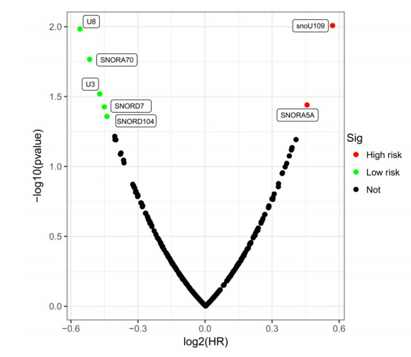
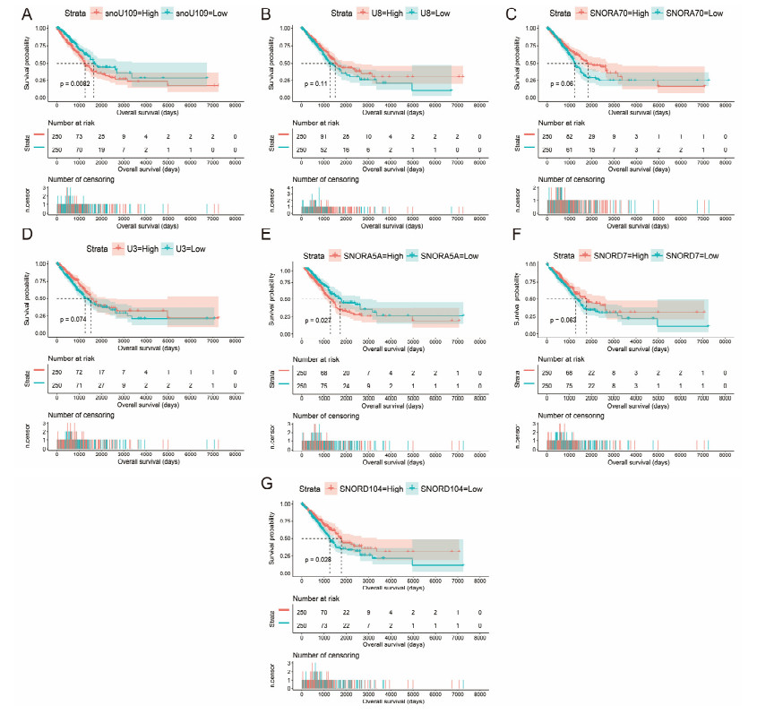
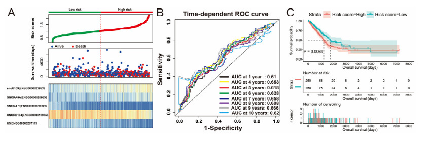
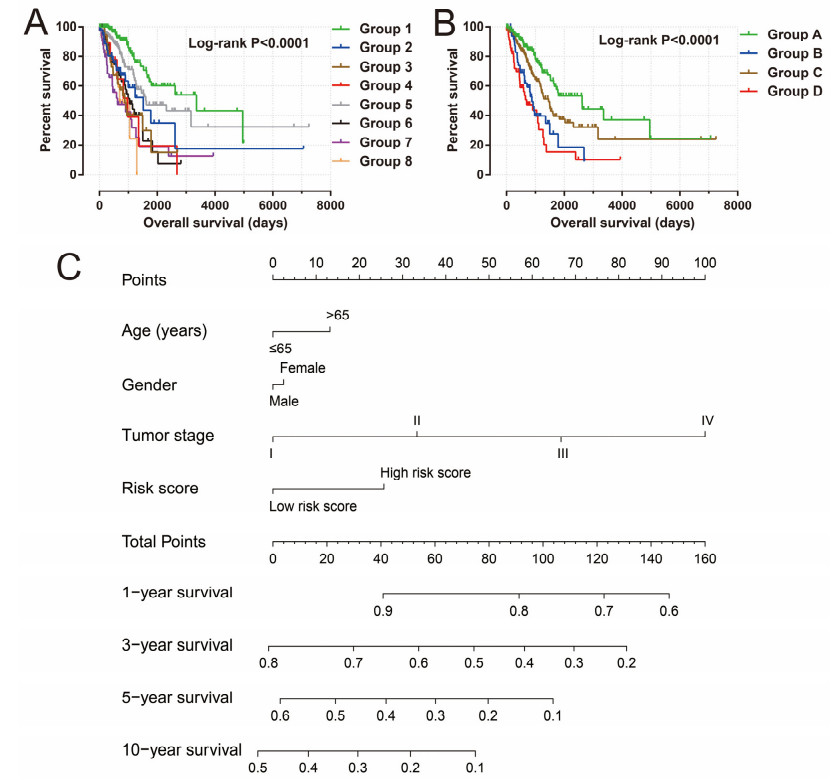
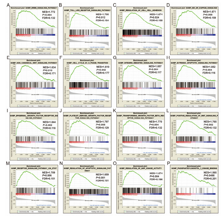
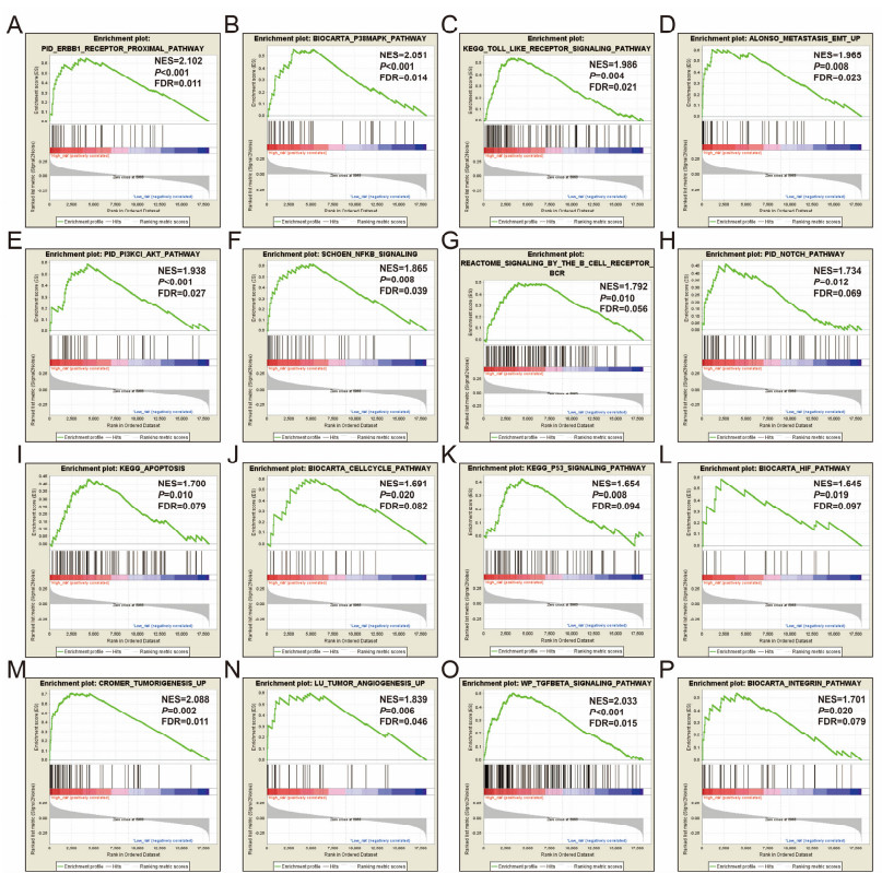
Since multiple studies have reported that small nucleolar RNAs (snoRNAs) can be serve as prognostic biomarkers for cancers, however, the prognostic values of snoRNAs in lung adenocarcinoma (LUAD) remain unclear. Therefore, the main work of this study is to identify the prognostic snoRNAs of LUAD and conduct a comprehensive analysis. The Cancer Genome Atlas LUAD cohort whole-genome RNA-sequencing dataset is included in this study, prognostic analysis and multiple bioinformatics approaches are used for comprehensive analysis and identification of prognostic snoRNAs. There were seven LUAD prognostic snoRNAs were screened in current study. We also constructed a novel expression signature containing five LUAD prognostic snoRNAs (snoU109, SNORA5A, SNORA70, SNORD104 and U3). Survival analysis of this expression signature reveals that LUAD patients with high risk score was significantly related to an unfavourable overall survival (adjusted P = 0.01, adjusted hazard ratio = 1.476, 95% confidence interval = 1.096-1.987). Functional analysis indicated that LUAD patients with different risk score phenotypes had significant differences in cell cycle, apoptosis, integrin, transforming growth factor beta, ErbB, nuclear factor kappa B, mitogen-activated protein kinase, phosphatidylinositol-3-kinase and toll like receptor signaling pathway. Immune microenvironment analysis also indicated that there were significant differences in immune microenvironment scores among LUAD patients with different risk score. In conclusion, this study identified an novel expression signature containing five LUAD prognostic snoRNAs, which may be serve as an independent prognostic indicator for LUAD patients.
Citation: Linbo Zhang, Mei Xin, Peng Wang. Identification of a novel snoRNA expression signature associated with overall survival in patients with lung adenocarcinoma: A comprehensive analysis based on RNA sequencing dataset[J]. Mathematical Biosciences and Engineering, 2021, 18(6): 7837-7860. doi: 10.3934/mbe.2021389
Since multiple studies have reported that small nucleolar RNAs (snoRNAs) can be serve as prognostic biomarkers for cancers, however, the prognostic values of snoRNAs in lung adenocarcinoma (LUAD) remain unclear. Therefore, the main work of this study is to identify the prognostic snoRNAs of LUAD and conduct a comprehensive analysis. The Cancer Genome Atlas LUAD cohort whole-genome RNA-sequencing dataset is included in this study, prognostic analysis and multiple bioinformatics approaches are used for comprehensive analysis and identification of prognostic snoRNAs. There were seven LUAD prognostic snoRNAs were screened in current study. We also constructed a novel expression signature containing five LUAD prognostic snoRNAs (snoU109, SNORA5A, SNORA70, SNORD104 and U3). Survival analysis of this expression signature reveals that LUAD patients with high risk score was significantly related to an unfavourable overall survival (adjusted P = 0.01, adjusted hazard ratio = 1.476, 95% confidence interval = 1.096-1.987). Functional analysis indicated that LUAD patients with different risk score phenotypes had significant differences in cell cycle, apoptosis, integrin, transforming growth factor beta, ErbB, nuclear factor kappa B, mitogen-activated protein kinase, phosphatidylinositol-3-kinase and toll like receptor signaling pathway. Immune microenvironment analysis also indicated that there were significant differences in immune microenvironment scores among LUAD patients with different risk score. In conclusion, this study identified an novel expression signature containing five LUAD prognostic snoRNAs, which may be serve as an independent prognostic indicator for LUAD patients.

| [1] |
T. Bratkovic, J. Bozic, B. Rogelj, Functional diversity of small nucleolar RNAs, Nucleic Acids Res., 48 (2020), 1627-1651. doi: 10.1093/nar/gkz1140

|
| [2] |
J. Gong, Y. Li, C. J. Liu, Y. Xiang, C. Li, Y. Ye, et al., A pan-cancer analysis of the expression and clinical relevance of small nucleolar RNAs in human cancer, Cell Rep., 21 (2017), 1968-1981. doi: 10.1016/j.celrep.2017.10.070
|
| [3] |
J. Liang, J. Wen, Z. Huang, X. P. Chen, B. X. Zhang, L. Chu, Small nucleolar RNAs: Insight into their function in cancer, Front. Oncol., 9 (2019), 587. doi: 10.3389/fonc.2019.00587
|
| [4] |
H. Shuwen, Y. Xi, Q. Quan, J. Yin, D. Miao, Can small nucleolar RNA be a novel molecular target for hepatocellular carcinoma?, Gene, 733 (2020), 144384. doi: 10.1016/j.gene.2020.144384
|
| [5] |
V. L. Dsouza, D. Adiga, S. Sriharikrishnaa, P. S. Suresh, A. Chatterjee, S. P. Kabekkodu, Small nucleolar RNA and its potential role in breast cancer-A comprehensive review, Biochem. Biophys. Acta Rev. Cancer, 1875 (2021), 188501. doi: 10.1016/j.bbcan.2020.188501
|
| [6] |
J. Liu, X. Liao, X. Zhu, P. Lv, R. Li, Identification of potential prognostic small nucleolar RNA biomarkers for predicting overall survival in patients with sarcoma, Cancer Med., 9 (2020), 7018-7033. doi: 10.1002/cam4.3361
|
| [7] |
T. Deng, Y. Gong, X. Liao, X. Wang, X. Zhou, G. Zhu, et al., Integrative analysis of a novel eleven-small nucleolar RNA prognostic signature in patients with lower grade glioma, Front. Oncol., 11 (2021), 650828. doi: 10.3389/fonc.2021.650828
|
| [8] |
Cancer Genome Atlas Research Network, Comprehensive molecular profiling of lung adenocarcinoma, Nature, 511 (2014), 543-550. doi: 10.1038/nature13385
|
| [9] | L. Zhang, G. Zhu, X. Wang, X. Liao, R. Huang, C. Huang, et al., Genomewide investigation of the clinical significance and prospective molecular mechanisms of kinesin family member genes in patients with lung adenocarcinoma, Oncol. Rep., 42 (2019), 1017-1034. |
| [10] |
A. Subramanian, P. Tamayo, V. K. Mootha, S. Mukherjee, B. L. Ebert, M. A. Gillette, et al., Gene set enrichment analysis: a knowledge-based approach for interpreting genome-wide expression profiles, Proc. Nat. Acad. Sci. U. S. A., 102 (2005), 15545-15550. doi: 10.1073/pnas.0506580102
|
| [11] |
A. Liberzon, C. Birger, H. Thorvaldsdottir, M. Ghandi, J. P. Mesirov, P. Tamayo, The molecular signatures database (MSigDB) hallmark gene set collection, Cell Syst., 1 (2015), 417-425. doi: 10.1016/j.cels.2015.12.004
|
| [12] |
G. Dennis, Jr., B. T. Sherman, D. A. Hosack, J. Yang, W. Gao, H. C. Lane, et al., DAVID: Database for annotation, visualization and integrated discovery, Genome Biol., 4 (2003), P3. doi: 10.1186/gb-2003-4-5-p3
|
| [13] |
X. Jiao, B. T. Sherman, W. H. Da, R. Stephens, M. W. Baseler, H. C. Lane, et al., DAVID-WS: a stateful web service to facilitate gene/protein list analysis, Bioinformatics, 28 (2012), 1805-1806. doi: 10.1093/bioinformatics/bts251
|
| [14] |
K. Yoshihara, M. Shahmoradgoli, E. Martinez, R. Vegesna, H. Kim, W. Torres-Garcia, et al., Inferring tumour purity and stromal and immune cell admixture from expression data, Nat. Commun., 4 (2013), 2612. doi: 10.1038/ncomms3612
|
| [15] |
Y. Benjamini, D. Drai, G. Elmer, N. Kafkafi, I. Golani, Controlling the false discovery rate in behavior genetics research, Behav. Brain Res., 125 (2001), 279-284. doi: 10.1016/S0166-4328(01)00297-2
|
| [16] | M. Esteller, Non-coding RNAs in human disease, Nat. Rev. Genet., 12 (2011), 861-874. |
| [17] |
G. Romano, D. Veneziano, M. Acunzo, C. M. Croce, Small non-coding RNA and cancer, Carcinogenesis, 38 (2017), 485-491. doi: 10.1093/carcin/bgx026
|
| [18] |
G. T. Williams, F. Farzaneh, Are snoRNAs and snoRNA host genes new players in cancer?, Nat. Rev. Cancer, 12 (2012), 84-88. doi: 10.1038/nrc3195
|
| [19] |
Y. Liu, H. Ruan, S. Li, Y. Ye, W. Hong, J. Gong, et al., The genetic and pharmacogenomic landscape of snoRNAs in human cancer, Mol. Cancer, 19 (2020), 108. doi: 10.1186/s12943-020-01228-z
|
| [20] |
R. Cao, B. Ma, L. Yuan, G. Wang, Y. Tian, Small nucleolar RNAs signature (SNORS) identified clinical outcome and prognosis of bladder cancer (BLCA), Cancer Cell Int., 20 (2020), 299. doi: 10.1186/s12935-020-01393-7
|
| [21] | X. Pan, L. Chen, K. Y. Feng, X. H. Hu, Y. H. Zhang, X. Y. Kong, et al., Analysis of expression pattern of snoRNAs in different cancer types with machine learning algorithms, Int. J. Mol. Sci., 20 (2019). |
| [22] |
Y. Zhao, Y. Yan, R. Ma, X. Lv, L. Zhang, J. Wang, et al., Expression signature of six-snoRNA serves as novel non-invasive biomarker for diagnosis and prognosis prediction of renal clear cell carcinoma, J. Cell Mol. Med., 24 (2020), 2215-2228. doi: 10.1111/jcmm.14886
|
| [23] | H. Yu, Z. Pang, G. Li, T. Gu, Bioinformatics analysis of differentially expressed miRNAs in non-small cell lung cancer, J. Clin. Lab. Anal., 35 (2021), e23588. |
| [24] |
H. Lin, B. Wang, J. Yu, J. Wang, Q. Li, B. Cao, Protein arginine methyltransferase 8 gene enhances the colon cancer stem cell (CSC) function by upregulating the pluripotency transcription factor, J. Cancer, 9 (2018), 1394-1402. doi: 10.7150/jca.23835
|
| [25] |
S. J. Hernandez, D. M. Dolivo, T. Dominko, PRMT8 demonstrates variant-specific expression in cancer cells and correlates with patient survival in breast, ovarian and gastric cancer, Oncol. Lett., 13 (2017), 1983-1989. doi: 10.3892/ol.2017.5671
|
| [26] |
C. Andolino, C. Hess, T. Prince, H. Williams, M. Chernin, Drug-induced keratin 9 interaction with Hsp70 in bladder cancer cells, Cell Stress Chaperones, 23 (2018), 1137-1142. doi: 10.1007/s12192-018-0913-2
|
| [27] | E. Anguita, F. J. Candel, A. Chaparro, J. J. Roldan-Etcheverry, Transcription factor GFI1B in health and disease, Front. Oncol., 7 (2017), 54. |
| [28] | A. N. Cheng, E. L. Bao, C. Fiorini, V. G. Sankaran, Macrothrombocytopenia associated with a rare GFI1B missense variant confounding the presentation of immune thrombocytopenia, Pediatr. Blood Cancer, 66 (2019), e27874. |
| [29] |
A. Thivakaran, L. Botezatu, J. M. Hones, J. Schutte, L. Vassen, Y. S. Al-Matary, et al., Gfi1b: a key player in the genesis and maintenance of acute myeloid leukemia and myelodysplastic syndrome, Haematologica, 103 (2018), 614-625. doi: 10.3324/haematol.2017.167288
|
| [30] |
E. Anguita, R. Gupta, V. Olariu, P. J. Valk, C. Peterson, R. Delwel, et al., A somatic mutation of GFI1B identified in leukemia alters cell fate via a SPI1 (PU.1) centered genetic regulatory network, Dev. Biol., 411 (2016), 277-286. doi: 10.1016/j.ydbio.2016.02.002
|
| [31] | M. Faleschini, N. Papa, M. C. Morel-Kopp, C. Marconi, T. Giangregorio, F. Melazzini, et al., Dysregulation of oncogenic factors by GFI1B p32: investigation of a novel GFI1B germline mutation, Haematologica, 2021. |
| [32] |
A. H. Elmaagacli, M. Koldehoff, J. L. Zakrzewski, N. K. Steckel, H. Ottinger, D. W. Beelen, Growth factor-independent 1B gene (GFI1B) is overexpressed in erythropoietic and megakaryocytic malignancies and increases their proliferation rate, Br. J. Haematol., 136 (2007), 212-219. doi: 10.1111/j.1365-2141.2006.06407.x
|
| [33] |
L. Vassen, C. Khandanpour, P. Ebeling, B. A. van der Reijden, J. H. Jansen, S. Mahlmann, et al., Growth factor independent 1b (Gfi1b) and a new splice variant of Gfi1b are highly expressed in patients with acute and chronic leukemia, Int. J. Hematol., 89 (2009), 422-430. doi: 10.1007/s12185-009-0286-5
|
 mbe-18-06-389-Supplementary tables.pdf mbe-18-06-389-Supplementary tables.pdf |
 |
Figures(17) / Tables(2)

Linbo Zhang, Mei Xin, Peng Wang. Identification of a novel snoRNA expression signature associated with overall survival in patients with lung adenocarcinoma: A comprehensive analysis based on RNA sequencing dataset[J]. Mathematical Biosciences and Engineering, 2021, 18(6): 7837-7860. doi: 10.3934/mbe.2021389


 DownLoad: