Emergent dynamics of various Cucker–Smale type models with a fractional derivative

Hyunjin Ahn; Myeongju Kang; Hyunjin Ahn; Myeongju Kang

doi:10.3934/mbe.2023798

Mathematical Biosciences and Engineering

2023, Volume 20, Issue 10: 17949-17985. doi: 10.3934/mbe.2023798

Previous Article Next Article

Research article Special Issues

Emergent dynamics of various Cucker–Smale type models with a fractional derivative

Hyunjin Ahn ^{1
,
,},
Myeongju Kang ²

1.
Department of Mathematics, Myongji University, Gyeonggi-do 17058, South Korea
2.
School of Mathematics, Korea Institute for Advanced Study, Seoul 02455, South Korea

Received: 28 July 2023 Revised: 06 September 2023 Accepted: 10 September 2023 Published: 19 September 2023

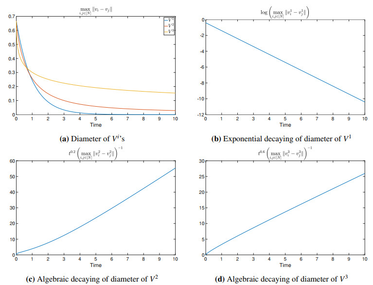
In this paper, we demonstrate emergent dynamics of various Cucker–Smale type models, especially standard Cucker–Smale (CS), thermodynamic Cucker–Smale (TCS), and relativistic Cucker–Smale (RCS) with a fractional derivative in time variable. For this, we adopt the Caputo fractional derivative as a widely used standard fractional derivative. We first introduce basic concepts and previous properties based on fractional calculus to explain its unusual aspects compared to standard calculus. Thereafter, for each proposed fractional model, we provide several sufficient frameworks for the asymptotic flocking of the proposed systems. Unlike the flocking dynamics which occurs exponentially fast in the original models, we focus on the flocking dynamics that occur slowly at an algebraic rate in the fractional systems.
- asymptotic flocking,
- Caputo fractional derivative,
- Cucker–Smale,
- relativistic Cucker–Smale,
- thermodynamic Cucker–Smale
Citation: Hyunjin Ahn, Myeongju Kang. Emergent dynamics of various Cucker–Smale type models with a fractional derivative[J]. Mathematical Biosciences and Engineering, 2023, 20(10): 17949-17985. doi: 10.3934/mbe.2023798

Related Papers:

Abstract

In this paper, we demonstrate emergent dynamics of various Cucker–Smale type models, especially standard Cucker–Smale (CS), thermodynamic Cucker–Smale (TCS), and relativistic Cucker–Smale (RCS) with a fractional derivative in time variable. For this, we adopt the Caputo fractional derivative as a widely used standard fractional derivative. We first introduce basic concepts and previous properties based on fractional calculus to explain its unusual aspects compared to standard calculus. Thereafter, for each proposed fractional model, we provide several sufficient frameworks for the asymptotic flocking of the proposed systems. Unlike the flocking dynamics which occurs exponentially fast in the original models, we focus on the flocking dynamics that occur slowly at an algebraic rate in the fractional systems.

References

[1]	J. Buck, E. Buck, Biology of synchronous flashing of fireflies, Nature, 211 (1966), 562–564. https://doi.org/10.1038/211562a0 doi: 10.1038/211562a0
[2]	G. B. Ermentrout, An adaptive model for synchrony in the firefly Pteroptyx malaccae, J. Math. Biol., 29 (1991), 571–585. https://doi.org/10.1007/BF00164052 doi: 10.1007/BF00164052
[3]	A. T. Winfree, Biological rhythms and the behavior of populations of coupled oscillators, J. Theor. Biol., 16 (1967), 15–42. https://doi.org/10.1016/0022-5193(67)90051-3 doi: 10.1016/0022-5193(67)90051-3
[4]	C. M. Topaz, A. L. Bertozzi, Swarming patterns in a two-dimensional kinematic model for biological groups, SIAM J. Appl. Math., 65 (2004), 152–174. https://doi.org/10.1137/S0036139903437424 doi: 10.1137/S0036139903437424
[5]	F. Cucker, S. Smale, Emergent behavior in flocks, IEEE Trans. Automat. Control, 52 (2007), 852–862. https://doi.org/10.1109/TAC.2007.895842 doi: 10.1109/TAC.2007.895842
[6]	P. Degond, S. Motsch, Large-scale dynamics of the persistent turning walker model of fish behavior, J. Stat. Phys., 131 (2008), 989–1022. https://doi.org/10.1007/s10955-008-9529-8 doi: 10.1007/s10955-008-9529-8
[7]	J. Toner, Y. Tu, Flocks, herds and schools: A quantitative theory of flocking, Phys. Rev. E, 58 (1998), 4828–4858.
[8]	J. A. Acebron, L. L. Bonilla, C. J. P. Pérez Vicente, F. Ritort, R. Spigler, The Kuramoto model: A simple paradigm for synchronization phenomena, Rev. Mod. Phys., 77 (2005), 137–185. https://doi.org/10.1103/RevModPhys.77.137 doi: 10.1103/RevModPhys.77.137
[9]	Y. P. Choi, S. Y. Ha, Z. Li, Emergent dynamics of the Cucker–Smale flocking model and its variants, in Active Particles Vol.I Theory, Models, Applications (tentative title), Series: Modeling and Simulation in Science and Technology, Birkhauser, Springer, 2017.
[10]	R. Olfati-Saber, Flocking for multi-agent dynamic systems: algorithms and theory, IEEE Trans. Automat. Contr., 51 (2006), 401–420. https://doi.org/10.1109/TAC.2005.864190 doi: 10.1109/TAC.2005.864190
[11]	A. Pikovsky, M. Rosenblum, J. Kurths, Synchronization: A Universal Concept in Nonlinear Sciences, Cambridge University Press, Cambridge, 2001.
[12]	S. H. Strogatz, From Kuramoto to Crawford: exploring the onset of synchronization in populations of coupled oscillators, Phys. D, 143 (2000), 1–20. https://doi.org/10.1016/S0167-2789(00)00094-4 doi: 10.1016/S0167-2789(00)00094-4
[13]	T. Vicsek, A. Zefeiris, Collective motion, Phys. Rep., 517 (2012), 71–140. https://doi.org/10.1016/j.physrep.2012.03.004 doi: 10.1016/j.physrep.2012.03.004
[14]	A. T. Winfree, The geometry of biological time, Springer, New York, 1980.
[15]	T. Vicsek, A. Czirók, E. Ben-Jacob, I. Cohen, O. Schochet, Novel type of phase transition in a system of self-driven particles, Phys. Rev. Lett., 75 (1995), 1226–1229. https://doi.org/10.1103/PhysRevLett.75.1226 doi: 10.1103/PhysRevLett.75.1226
[16]	H. Ahn, S. Y. Ha, D. Kim, F. Schlöder, W. Shim, The mean-field limit of the Cucker–Smale model on Riemannian manifolds, Q. Appl. Math., 80 (2022), 403–450. https://doi.org/10.1090/qam/1613 doi: 10.1090/qam/1613
[17]	S. Y. Ha, J. G. Liu, A simple proof of Cucker–Smale flocking dynamics and mean-field limit, Commun. Math. Sci., 7 (2009), 297–325.
[18]	S. Y. Ha, J. Kim, X. Zhang, Uniform stability of the Cucker–Smale model and its application to the mean-field limit, Kinet. Relat. Models, 11 (2018), 1157–1181. https://doi.org/10.3934/krm.2018045 doi: 10.3934/krm.2018045
[19]	J. A. Carrillo, M. Fornasier, J. Rosado, G. Toscani, Asymptotic flocking dynamics for the kinetic Cucker–Smale model, SIAM. J. Math. Anal., 42 (2010), 218–236. https://doi.org/10.1137/090757290 doi: 10.1137/090757290
[20]	S. Y. Ha, E. Tadmor, From particle to kinetic and hydrodynamic description of flocking, Kinet. Relat. Models, 1 (2008), 415–435.
[21]	A. Figalli, M. Kang, A rigorous derivation from the kinetic Cucker–Smale model to the pressureless Euler system with nonlocal alignment, Anal. PDE., 12 (2019), 843–866. https://doi.org/10.2140/apde.2019.12.843 doi: 10.2140/apde.2019.12.843
[22]	S. Y. Ha, M. J Kang, B. Kwon, A hydrodynamic model for the interaction of Cucker–Smale particles and incompressible fluid, Math. Models. Methods Appl. Sci., 11 (2014), 2311–2359. https://doi.org/10.1142/S0218202514500225 doi: 10.1142/S0218202514500225
[23]	T. K. Karper, A. Mellet, K. Trivisa, Hydrodynamic limit of the kinetic Cucker–Smale flocking model, Math. Models Methods Appl. Sci., 25 (2015), 131–163. https://doi.org/10.1142/S0218202515500050 doi: 10.1142/S0218202515500050
[24]	Y. P. Choi, Z. Li, Emergent behavior of Cucker–Smale flocking particles with heterogeneous time delays, Appl. Math. Lett., 86 (2018), 49–56. https://doi.org/10.1016/j.aml.2018.06.018 doi: 10.1016/j.aml.2018.06.018
[25]	P. Cattiaux, F. Delebecque, L. Pedeches, Stochastic Cucker–Smale models: old and new, Ann. Appl. Probab., 28 (2018), 3239–3286. https://doi.org/10.1214/18-AAP1400 doi: 10.1214/18-AAP1400
[26]	J. Cho, S. Y. Ha, F. Huang, C. Jin, D. Ko, Emergence of bi-cluster flocking for the Cucker–Smale model, Math. Models Methods Appl. Sci., 26 (2016), 1191–1218. https://doi.org/10.1142/S0218202516500287 doi: 10.1142/S0218202516500287
[27]	S. H. Choi, S. Y. Ha, Emergence of flocking for a multi-agent system moving with constant speed, Commun. Math. Sci., 14 (2016), 953–972.
[28]	Y. P. Choi, D. Kalsie, J. Peszek, A. Peters, A collisionless singular Cucker–Smale model with decentralized formation control, SIAM J. Appl. Dyn. Syst., 18 (2019), 1954–1981. https://doi.org/10.1137/19M1241799 doi: 10.1137/19M1241799
[29]	I. Podlubny, Fractional differential equations: An introduction to fractional derivatives, fractional differential equations, to methods of their solution and some of their applications, in Mathematics in Science and Engineering, Academic press, 198 (1999).
[30]	G. R. J. Cooper, D. R. Cowan, Filtering using variable order vertical derivatives, Comput. Geosci., 30 (2004), 455–459. https://doi.org/10.1016/j.cageo.2004.03.001 doi: 10.1016/j.cageo.2004.03.001
[31]	E. Girejko, D. Mozyrska, M. Wyrwas, Numerical analysis of behaviour of the Cucker–Smale type models with fractional operators, J. Comput. Appl. Math, 339 (2018), 111–123. https://doi.org/10.1016/j.cam.2017.12.013 doi: 10.1016/j.cam.2017.12.013
[32]	E. Girejko, D. Mozyrska, M. Wyrwas, On the fractional variable order Cucker–Smale type model, IFAC-PapersOnLine, 51 (2018), 693–697. https://doi.org/10.1016/j.ifacol.2018.06.184 doi: 10.1016/j.ifacol.2018.06.184
[33]	A. B. Malinowska, T. Odzijewicz, E. Schmeidel, On the existence of optimal controls for the fractional continuous-time Cucker–Smale model, in Theory and Applications of Non-integer Order Systems (eds. A. Babiarz, A. Czornik, J. Klamka and M. Niezabitowski), Springer International Publishing, (2017), 227–240. https://doi.org/10.1007/978-3-319-45474-0
[34]	R. Almeida, R. Kamocki, A. B. Malinowska, T. Odzijewicz, On the necessary optimality conditions for the fractional Cucker–Smale optimal control problem, Commun. Nonlinear Sci. Numer. Simul., 96 (2021), 105678. https://doi.org/10.1016/j.cnsns.2020.105678 doi: 10.1016/j.cnsns.2020.105678
[35]	R. Almeida, R. Kamocki, A. B. Malinowska, T. Odzijewicz, On the existence of optimal consensus control for the fractional Cucker-Smale model, Arch. Control Sci., 30 (2020), 625–651.
[36]	S. Y. Ha, J. Jung, P. Kuchling, Emergence of anomalous flocking in the fractional Cucker–Smale model, Discrete Contin. Dyn. Syst., 39 (2019), 5465–5489. https://doi.org/10.3934/dcds.2019223 doi: 10.3934/dcds.2019223
[37]	J. G. Dong, S. Y. Ha, D. Kim, Emergent behaviors of continuous and discrete thermomechanical Cucker–Smale models on general digraphs, Math. Models. Methods Appl. Sci., 29 (2019), 589–632. https://doi.org/10.1142/S0218202519400013 doi: 10.1142/S0218202519400013
[38]	J. G. Dong, S. Y. Ha, J. Jung, D. Kim, On the stochastic flocking of the Cucker–Smale flock with randomly switching topologies, SIAM J. Control. Optim., 58 (2020), 2332–2353. https://doi.org/10.1137/19M1279150 doi: 10.1137/19M1279150
[39]	S. Y. Ha, T. Ruggeri, Emergent dynamics of a thermodynamically consistent particle model, Arch. Ration. Mech. Anal., 223 (2017), 1397–1425.
[40]	S. Y. Ha, J. Kim, T. Ruggeri, Emergent behaviors of thermodynamic Cucker-Smale particles, SIAM J. Math. Anal., 50 (2019), 3092–3121. https://doi.org/10.1137/17M111064X doi: 10.1137/17M111064X
[41]	S. Y. Ha, J. Kim, C. Min, T. Ruggeri, X. Zhang, Uniform stability and mean-field limit of a thermodynamic Cucker–Smale model, Quart. Appl. Math., 77 (2019), 131–176. https://doi.org/10.1090/qam/1517 doi: 10.1090/qam/1517
[42]	S. Y. Ha, M. J Kang, J. Kim, W. Shim, Hydrodynamic limit of the kinetic thermomechanical Cucker–Smale model in a strong local alignment regime, Commun. Pure Appl. Anal., 19 (2019), 1233–1256. https://doi.org/10.3934/cpaa.2020057 doi: 10.3934/cpaa.2020057
[43]	H. Cho, J. G. Dong, S. Y. Ha, Emergent behaviors of a thermodynamic Cucker–Smale flock with a time delay on a general digraph, Math. Methods Appl. Sci., 45 (2021), 164–196. https://doi.org/10.1002/mma.7771 doi: 10.1002/mma.7771
[44]	H. Ahn, S. Y. Ha, W. Shim, Emergent dynamics of a thermodynamic Cucker–Smale ensemble on complete Riemannian manifolds, Kinet. Relat. Models, 14 (2021), 323–351. https://doi.org/10.3934/krm.2021007 doi: 10.3934/krm.2021007
[45]	S. Y. Ha, J. Kim, T. Ruggeri, From the relativistic mixture of gases to the relativistic Cucker–Smale flocking, Arch. Rational Mech. Anal., 235 (2020), 1661–1706. https://doi.org/10.1007/s00205-019-01452-y doi: 10.1007/s00205-019-01452-y
[46]	H. Ahn, S. Y. Ha, J. Kim, Uniform stability of the relativistic Cucker–Smale model and its application to a mean-field limit, Commun. Pure Appl. Anal., 20 (2021), 4209–4237. https://doi.org/10.3934/cpaa.2021156 doi: 10.3934/cpaa.2021156
[47]	H. Ahn, S. Y. Ha, M. Kang, W. Shim, Emergent behaviors of relativistic flocks on Riemannian manifolds, Phys. D., 427 (2021), 133011. https://doi.org/10.1016/j.physd.2021.133011 doi: 10.1016/j.physd.2021.133011
[48]	J. Byeon, S. Y. Ha, J. Kim, Asymptotic flocking dynamics of a relativistic Cucker–Smale flock under singular communications, J. Math. Phys., 63 (2022), 012702. https://doi.org/10.1063/5.0062745 doi: 10.1063/5.0062745
[49]	H. Ahn, S. Y. Ha, J. Kim, Nonrelativistic limits of the relativistic Cucker–Smale model and its kinetic counterpart, J. Math. Phys., 63 (2022), 082701. https://doi.org/10.1063/5.0070586 doi: 10.1063/5.0070586
[50]	H. Ahn, Asymptotic flocking of the relativistic Cucker–Smale model with time delay, Netw. Heterog. Media, 18 (2023), 29-47. https://doi.org/10.3934/nhm.2023002 doi: 10.3934/nhm.2023002
[51]	S. Y. Ha, J. Kim, T. Ruggeri, Kinetic and hydrodynamic models for the relativistic Cucker–Smale ensemble and emergent dynamics, Commun. Math. Sci., 19 (2021), 1945–1990.
[52]	M. Merkle, Completely monotone functions, A digest, in Analytic Number theory, Approximation Theory, and Special Functions (eds. G. V. Milovanović and M. Th. Rassias), Springer New York, (2014), 577–621.
[53]	W. R. Schneider, Completely monotone generalized Mittag-Leffler functions, Expo. Math., 14 (1996), 3–16.
[54]	K. Diethelm, Monotonocity of functions and sign changes of their Caputo derivatives, Fract. Calc. Appl. Anal., 19 (2016), 561–566.
[55]	B. Bonilla, M. Rivero, J. J. Trujillo, On systems of linear fractional differential equations with constant coefficients, Appl. Math. Comput., 187 (2007), 68–78. https://doi.org/10.1016/j.amc.2006.08.104 doi: 10.1016/j.amc.2006.08.104
[56]	L. Bourdin, Cauchy–Lipschitz theory for fractional multi-order dynamics: State-transition matrices, Duhamel formulas and duality theorems, Differ. Integral Equation, 31 (2018), 559–594.
[57]	B. Piccoli, F. Rossi, E. Trélat, Control to flocking of the kinetic Cucker–Smale model, SIAM J. Math. Anal., 47 (2014), 4685–4719. https://doi.org/10.1137/140996501 doi: 10.1137/140996501

Reader Comments

Your name:*

Email:*
© 2023 the Author(s), licensee AIMS Press. This is an open access article distributed under the terms of the Creative Commons Attribution License (http://creativecommons.org/licenses/by/4.0)