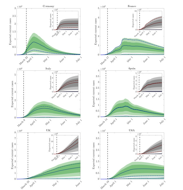
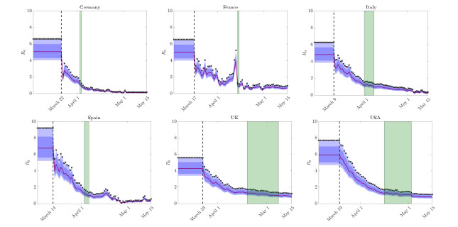
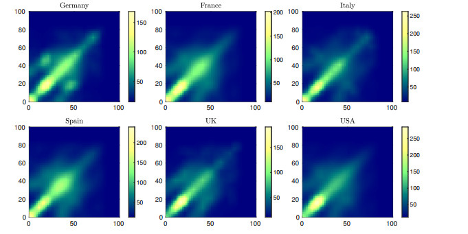
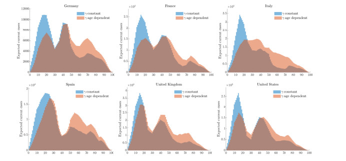
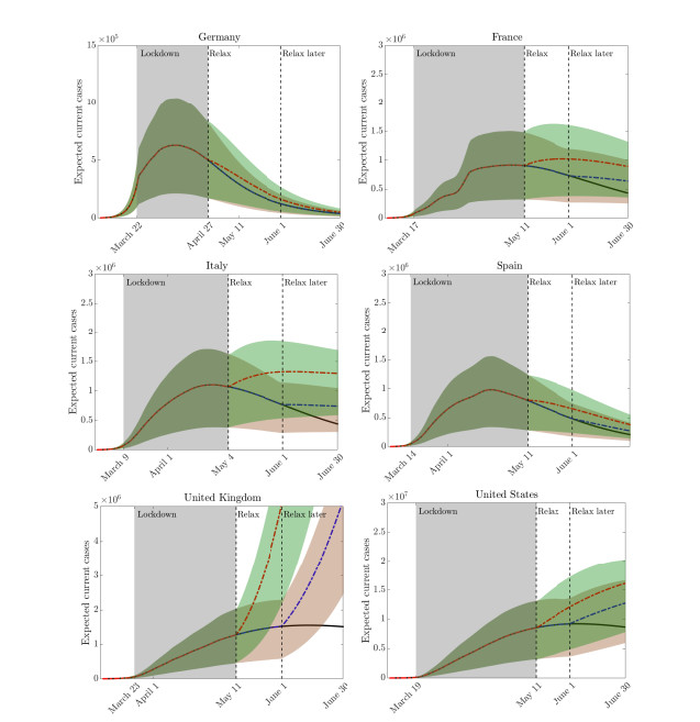
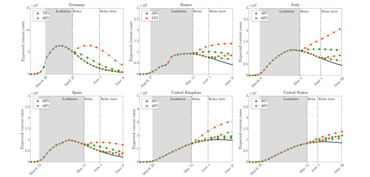
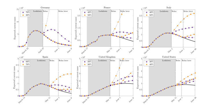
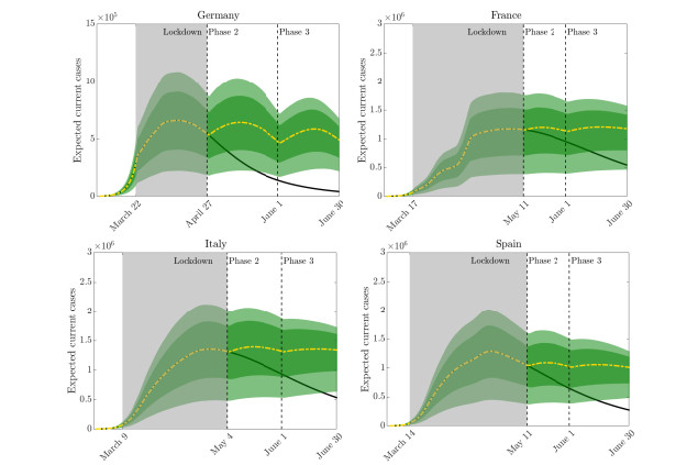
After the introduction of drastic containment measures aimed at stopping the epidemic contagion from SARS-CoV2, many governments have adopted a strategy based on a periodic relaxation of such measures in the face of a severe economic crisis caused by lockdowns. Assessing the impact of such openings in relation to the risk of a resumption of the spread of the disease is an extremely difficult problem due to the many unknowns concerning the actual number of people infected, the actual reproduction number and infection fatality rate of the disease. In this work, starting from a SEIRD compartmental model with a social structure based on the age of individuals and stochastic inputs that account for data uncertainty, the effects of containment measures are introduced via an optimal control problem dependent on specific social activities, such as home, work, school, etc. Through a short time horizon approximation, we derive models with multiple feedback controls depending on social activities that allow us to assess the impact of selective relaxation of containment measures in the presence of uncertain data. After analyzing the effects of the various controls, results from different scenarios concerning the first wave of the epidemic in some major countries, including Germany, France, Italy, Spain, the United Kingdom and the United States, are presented and discussed. Specific contact patterns in the home, work, school and other locations have been considered for each country. Numerical simulations show that a careful strategy of progressive relaxation of containment measures, such as that adopted by some governments, may be able to keep the epidemic under control by restarting various productive activities.
Citation: Giacomo Albi, Lorenzo Pareschi, Mattia Zanella. Modelling lockdown measures in epidemic outbreaks using selective socio-economic containment with uncertainty[J]. Mathematical Biosciences and Engineering, 2021, 18(6): 7161-7190. doi: 10.3934/mbe.2021355
After the introduction of drastic containment measures aimed at stopping the epidemic contagion from SARS-CoV2, many governments have adopted a strategy based on a periodic relaxation of such measures in the face of a severe economic crisis caused by lockdowns. Assessing the impact of such openings in relation to the risk of a resumption of the spread of the disease is an extremely difficult problem due to the many unknowns concerning the actual number of people infected, the actual reproduction number and infection fatality rate of the disease. In this work, starting from a SEIRD compartmental model with a social structure based on the age of individuals and stochastic inputs that account for data uncertainty, the effects of containment measures are introduced via an optimal control problem dependent on specific social activities, such as home, work, school, etc. Through a short time horizon approximation, we derive models with multiple feedback controls depending on social activities that allow us to assess the impact of selective relaxation of containment measures in the presence of uncertain data. After analyzing the effects of the various controls, results from different scenarios concerning the first wave of the epidemic in some major countries, including Germany, France, Italy, Spain, the United Kingdom and the United States, are presented and discussed. Specific contact patterns in the home, work, school and other locations have been considered for each country. Numerical simulations show that a careful strategy of progressive relaxation of containment measures, such as that adopted by some governments, may be able to keep the epidemic under control by restarting various productive activities.

| [1] |
G. Dimarco, L. Pareschi, G. Toscani, M. Zanella, Wealth distribution under the spread of infectious diseases, Phys. Rev. E, 102 (2020), 022303. doi: 10.1103/PhysRevE.102.022303

|
| [2] | C. Favero, A. Ichino, A. Rustichini, Restarting the Economy While Saving Lives Under COVID-19, CEPR Discussion Paper No. DP14664, 2020, Available from: https://ssrn.com/abstract = 3580626. |
| [3] |
M. Gatto, E. Bertuzzo, L. Mari, S. Miccoli, L. Carraro, R. Casagrandi, et al., Spread and dynamics of the COVID-19 epidemic in Italy: Effects of emergency containment measures, PNAS, 117 (2020), 10484–10491. doi: 10.1073/pnas.2004978117
|
| [4] |
S. Khajanchi, K. Sarkar, Forecasting the daily and cumulative number of cases for the COVID-19 pandemic in India, Chaos, 30 (2020), 071101. doi: 10.1063/5.0016240
|
| [5] |
S. Khajanchi, S. Bera, T. K. Roy, Mathematical analysis of the global dynamics of a HTLV-I infection model, considering the role of cytotoxic T-lymphocytes, Math. Comput. Simul., 180 (2021), 354–378. doi: 10.1016/j.matcom.2020.09.009
|
| [6] |
Q. Lin, S. Zhao, D. Gao, Y. Lou, S. Yang, S. S. Musa, et al., A conceptual model for the coronavirus disease 2019 (COVID-19) outbreak in Wuhan, China with individual reaction and governmental action, Int. J. Infect. Dis., 93 (2020), 211–216. doi: 10.1016/j.ijid.2020.02.058
|
| [7] |
P. Samui, J. Mondal, S. Khajanchi, A mathematical model for COVID-19 transmission dynamics with a case study of India, Chaos Solit. Fractals., 140 (2020), 110173. doi: 10.1016/j.chaos.2020.110173
|
| [8] |
B. Tang, X. Wang, Q. Li, N. L. Bragazzi, S. Tang, Y. Xiao, et al., Estimation of the Transmission Risk of the 2019-nCoV and Its Implication for Public Health Interventions, J. Clin. Med., 9 (2020), 462. doi: 10.3390/jcm9020462
|
| [9] |
B. Buonomo, R. Della Marca, Effects of information-induced behavioural changes during the COVID-19 lockdowns: the case of Italy, R. Soc. Open Sci., 7 (2020), 201635. doi: 10.1098/rsos.201635
|
| [10] | R. K. Rai, S. Khajanchi, P. K. Tiwari, E. Venturino, A. K. Misra, Impact of social media advertisements on the transmission dynamics of COVID-19 pandemic in India, J. Appl. Math. Comput., (2021), 1-26. |
| [11] |
C. Castillo-Chavez, H. W. Hethcote, V. Andreasen, S. A. Levin, W. M. Liu, Epidemiological models with age structure, proportionate mixing, and cross-immunity, J. Math. Biol., 27 (1989), 233–258. doi: 10.1007/BF00275810
|
| [12] |
A. Franceschetti, A. Pugliese, Threshold behaviour of a SIR epidemic model with age structure and immigration, J. Math. Biol., 57 (2008), 1–27. doi: 10.1007/s00285-007-0143-1
|
| [13] | H. W. Hethcote, Modeling heterogeneous mixing in infectious disease dynamics, In Models for Infectious Human Diseases, (eds. V. Isham and G. F. H. Medley), Cambridge University Press, Cambridge, UK, (1996), pp. 215–238. |
| [14] |
H. W. Hethcote, The mathematics of infectious diseases, SIAM Rev., 42 (2000), 599–653. doi: 10.1137/S0036144500371907
|
| [15] |
M. Iannelli, F. A. Milner, A. Pugliese, Analytical and numerical results for the age-structured S-I-S epidemic model with mixed inter-intracohort transmission, SIAM J. Math. Anal., 23 (1992), 662–688. doi: 10.1137/0523034
|
| [16] |
K. M. A. Kabir, J. Tanimoto, Evolutionary game theory modelling to represent the behavioural dynamics of economic shutdowns and shield immunity in the COVID-19 pandemic, R. Soc. Open Sci., 7 (2020), 201095. doi: 10.1098/rsos.201095
|
| [17] |
W. O. Kermack, A. G. McKendrick, A Contribution to the Mathematical Theory of Epidemics, Proc. Roy. Soc. Lond. A, 115 (1927), 700–721. doi: 10.1098/rspa.1927.0118
|
| [18] |
G. Albi, M. Herty, L. Pareschi, Kinetic description of optimal control problems and applications to opinion consensus, Commun. Math. Sci., 13 (2015), 1407–1429. doi: 10.4310/CMS.2015.v13.n6.a3
|
| [19] | G. Albi, L. Pareschi, Selective model-predictive control for flocking systems, Commun. Appl. Ind. Math., 9 (2018), 4–21. |
| [20] | G. Albi, L. Pareschi, M. Zanella, Uncertainty quantification in control problems for flocking models, Math. Probl. Eng., 2015 (2015), ID 850124. |
| [21] |
M. Bongini, M. Fornasier, D. Kalise, (Un)conditional consensus emergence under perturbed and decentralized feedback controls, Discrete Contin. Dyn. Syst., 35 (2015), 4071–4094. doi: 10.3934/dcds.2015.35.4071
|
| [22] | G. Dimarco, B. Perthame, G. Toscani, M. Zanella, Kinetic models for epidemic dynamics with social heterogeneity, J. Math. Biol., 83 (2021), 1–32. |
| [23] | B. Düring, L. Pareschi, G. Toscani, Kinetic models for optimal control of wealth inequalities, Eur. Phys. J. B, 91 (2018), Article No. 265. |
| [24] |
Z. Wang, C. T. Bauch, S. Bhattacharyya, A. d'Onofrio, P. Manfredi, M. Perc, et al., Statistical physics of vaccination, Phys. Rep., 664 (2016), 1–113. doi: 10.1016/j.physrep.2016.10.006
|
| [25] | K. Jagodnik, F. Ray, F. M. Giorgi, A. Lachmann, Correcting under-reported COVID-19 case numbers: estimating the true scale of the pandemic, (2020), in press. |
| [26] | K. Mizumoto, K. Kagaya, A. Zarebski, G. Chowell, Estimating the asymptomatic proportion of coronavirus disease 2019 (COVID-19) cases on board the Diamond Princess cruise ship, Yokohama, Japan, 2020, Euro. Surveill., 25 (2020), 2000180. |
| [27] |
S. Zhang, M. Diao, W. Yu, L. Pei, Z. Lin, D. Chen, Estimation of the reproductive number of novel coronavirus (COVID-19) and the probable outbreak size on the Diamond Princess cruise ship: A data-driven analysis, Int. J. Infect. Dis., 93 (2020), 201–204. doi: 10.1016/j.ijid.2020.02.033
|
| [28] |
G. Béraud, S. Kazmercziak, P. Beutels, D. Levy-Bruhl, X. Lenne, N. Mielcarek, et al., The French connection: The first large population-based contact survey in France relevant for the spread of infectious diseases, PLoS ONE, 10 (2015), e0133203. doi: 10.1371/journal.pone.0133203
|
| [29] |
J. Glasser, Z. Feng, A. Moylan, S. Del Valle, C. Castillo-Chavez, Mixing in age-structured population models of infectious diseases, Math. Bios., 235 (2012), 1–7. doi: 10.1016/j.mbs.2011.10.001
|
| [30] |
K. M. A. Kabir, T. Risa, J. Tanimoto, Prosocial behavior of wearing a mask during an epidemic: an evolutionary explanation, Scientific Reports, 11 (2021), 12621. doi: 10.1038/s41598-021-92094-2
|
| [31] |
J. Mossong, N. Hens, M. Jit, P. Beutels, K. Auranen, R. Mikolajczyk, et al., Social contacts and mixing patterns relevant to the spread of infectious diseases, PLoS Med., 5 (2008), e75. doi: 10.1371/journal.pmed.0050075
|
| [32] | K. Prem, A. R. Cook, M. Jit, Projecting social contact matrices in 152 countries using contact surveys and demographic data, PLoS ONE, 13 (2017), e1005697. |
| [33] |
A. Capaldi, S. Behrend, B. Berman, J. Smith, J. Wright, A. L. Lloyd, Parameter estimation and uncertainty quantification for an epidemic model, Math. Biosci. Eng., 9 (2012), 553–576. doi: 10.3934/mbe.2012.9.553
|
| [34] |
M. A. Capistrán, J. A. Christen, J. X. Velasco-Hernández, Towards uncertainty quantification and inference in the stochastic SIR epidemic model, Math. Biosci., 240 (2012), 250–259. doi: 10.1016/j.mbs.2012.08.005
|
| [35] | G. Chowell, Fitting dynamic models to epidemic outbreaks with quantified uncertainty: A primer for parameter uncertainty, identifiability, and forecasts, Infect. Dis. Model., 2 (2017), 379–398. |
| [36] |
M. G. Roberts, Epidemic models with uncertainty in the reproduction, J. Math. Biol., 66 (2013), 1463–1474. doi: 10.1007/s00285-012-0540-y
|
| [37] |
G. Albi, L. Pareschi, M. Zanella, Control with uncertain data of socially structured compartmental epidemic models, J. Math. Biol., 82 (2021), 1–41. doi: 10.1007/s00285-021-01560-y
|
| [38] | G. Dimarco, L. Pareschi, M. Zanella, Uncertainty quantification for kinetic models in socio-economic and life sciences. In Uncertainty Quantification for Hyperbolic and Kinetic Equations, (Eds. S. Jin, and L. Pareschi), SEMA SIMAI Springer Series, vol. 14, (2017), 151–191. |
| [39] | L. Pareschi, An introduction to uncertainty quantification for kinetic equations and related problems, In Trails in Kinetic Theory: Foundational Aspects and Numerical Methods, (Eds. G. Albi, S. Merino-Aceituno, A. Nota, M. Zanella), SEMA-SIMAI Springer Series vol. 25, (2021), 141–181. |
| [40] | D. Xiu, Numerical Methods for Stochastic Computations: A Spectral Methods Approach, Princeton University Press, 2010. |
| [41] |
M. Barro, A. Guiro, D. Ouedraogo, Optimal control of a SIR epidemic model with general incidence function and a time delays, Cubo, 20 (2018), 53–66. doi: 10.4067/S0719-06462018000200053
|
| [42] |
L. Bolzoni, E. Bonacini, C. Soresina, M. Groppi, Time-optimal control strategies in SIR epidemic models, Math. Biosci., 292 (2017), 86–96. doi: 10.1016/j.mbs.2017.07.011
|
| [43] | R. M. Colombo, M. Garavello, Optimizing vaccination strategies in an age structured SIR model, Math. Bios. Eng., 17 (2019), 1074–1089. |
| [44] |
A. d'Onofrio, P. Manfredi, E. Salinelli, Vaccinating behaviour, information, and the dynamics of SIR vaccine preventable diseases, Theor. Popul. Biol., 71 (2007), 301–317. doi: 10.1016/j.tpb.2007.01.001
|
| [45] | E. Franco, A feedback SIR (fSIR) model highlights advantages and limitations of infection-based social distancing, arXiv preprint arXiv: 2004.13216 (2020). |
| [46] |
S. Lee, G. Chowell, C. Castillo-Chávez, Optimal control for pandemic influenza: the role of limited antiviral treatment and isolation, J. Theor. Biol., 265 (2010), 136–150. doi: 10.1016/j.jtbi.2010.04.003
|
| [47] |
S. Lee, M. Golinski, G. Chowell, Modeling optimal age-specific vaccination strategies against pandemic influenza, Bull. Math. Biol., 74 (2012), 958–980. doi: 10.1007/s11538-011-9704-y
|
| [48] |
R. Dutta, S. Gomes, D. Kalise, L. Pacchiardi, Using mobility data in the design of optimal lockdown strategies for the COVID-19 pandemic, PLOS Comput. Biol., 17 (2021), e1009236. doi: 10.1371/journal.pcbi.1009236
|
| [49] | S. Flaxman, S. Mishra, A. Gandy, H. Unwin, H. Coupland, T. Mellan, et al., Estimating the number of infections and the impact of non-pharmaceutical interventions on COVID-19 in 11 European countries, Report 13. Imperial College COVID-19 Response Team, 30 March 2020. |
| [50] | S. Khajanchi, K. Sarkar, J. Mondal, K. S. Nisar, S. F. Abdelwahab, Mathematical modeling of the COVID-19 pandemic with intervention strategies, Res. Phys., 25 (2021), 104285. |
| [51] |
F. Lin, K. Muthuraman, M. Lawley, An optimal control theory approach to non-pharmaceutical interventions, BMC Infect. Dis., 10 (2010), 32. doi: 10.1186/1471-2334-10-32
|
| [52] | D. H. Morris, F. W. Rossine, J. B. Plotkin, S. A. Levin, Optimal, near-optimal, and robust epidemic control, Commun. Phys., 4 (2021), 1–8. |
| [53] |
G. Bertaglia, L. Pareschi, Hyperbolic models for the spread of epidemics on networks: kinetic description and numerical methods, ESAIM: Math. Model. Numer. Anal., 55 (2021), 381–407. doi: 10.1051/m2an/2020082
|
| [54] | G. Bertaglia, L. Pareschi, Hyperbolic compartmental models for epidemic spread on networks with uncertain data: application to the emergence of COVID-19 in Italy, Math. Mod. Meth. App. Sci., (2021), in press. |
| [55] | W. Boscheri, G. Dimarco, L. Pareschi, Modeling and simulating the spatial spread of an epidemic through multiscale kinetic equations, Math. Mod. Meth. App. Sci., (2021), 1–39. |
| [56] |
V. Capasso, G. Serio, A generalization of the Kermack-McKendrick deterministic epidemic model, Math. Biosci., 42 (1978), 43–61. doi: 10.1016/0025-5564(78)90006-8
|
| [57] |
J. Chen, H. Lu, G. Melino, S. Boccia, M. Piacentini, W. Ricciardi, et al., COVID-19 infection: the China and Italy perspectives, Cell Death Dis., 11 (2020), 1–17. doi: 10.1038/s41419-019-2182-0
|
| [58] |
E. Dong, H. Du, L. Gardner, An interactive web-based dashboard to track COVID-19 in real time, Lancet Infect. Dis., 20 (2020), 533–534. doi: 10.1016/S1473-3099(20)30120-1
|
| [59] |
G. Giordano, F. Blanchini, R. Bruno, P. Colaneri, A. Di Filippo, A. Di Matteo, et al., Modelling the COVID-19 epidemic and implementation of population-wide interventions in Italy, Nat. Med., 26 (2020), 855–860. doi: 10.1038/s41591-020-0883-7
|
| [60] |
A. Korobeinikov, P. K. Maini, Non-linear incidence and stability of infectious disease models, Math. Med. Biol., 22 (2005), 113–128. doi: 10.1093/imammb/dqi001
|
| [61] |
E. Lavezzo, E. Franchin, C. Ciavarella, G. Cuomo-Dannenburg, L. Barzon, C. Del Vecchio, et al., Suppression of a SARS-CoV-2 outbreak in the Italian municipality of Vo', Nature, 584 (2020), 425–429, doi: 10.1038/s41586-020-2488-1
|
| [62] |
X. Liu, P. Stechlinski, Infectious disease models with time-varying parameters and general nonlinear incidence rate, Appl. Math. Model., 36 (2012), 1974–1994. doi: 10.1016/j.apm.2011.08.019
|
| [63] | Y. Liu, A. A. Gayle, A. Wilder-Smith, J. Rocklöv, The reproductive number of COVID-19 is higher compared to SARS coronavirus, J. Travel Med., 27 (2020), 1–4. |
| [64] | G. Rinaldi, M. Paradisi, An empirical estimate of the infection fatality rate of COVID-19 from the first Italian outbreak, (2020), in press. |
| [65] | T. W. Russell, J. Hellewell, C. I. Jarvis, K. van Zandvoort, S. Abbott, R. Ratnayake, et al., Estimating the infection and case fatality ratio for coronavirus disease (COVID-19) using age-adjusted data from the outbreak on the Diamond Princess cruise ship, Euro. Surveill., 25 (2020), 2000256. |
| [66] | X. Tang, S. S. Musa, S. Zhao, S. Mei, D. He, Using Proper Mean Generation Intervals in Modeling of COVID-19, Front. Public Health, 9 (2020), 691262. |
| [67] |
S. Wang, F. Zhong, W. Bao, Y. Li, L. Liu, H. Wang, et al., Age-dependent risks of Incidence and Mortality of COVID- 19 in Hubei Province and Other Parts of China Hongdou, Front. Med., 7 (2020), 190. doi: 10.3389/fmed.2020.00190
|
| [68] |
M. Zanella, C. Bardelli, M. Azzi, S. Deandrea, P. Perotti, S. Silva, et al., Social contacts, epidemic spreading and health system. Mathematical modeling and applications to COVID-19 infection, Math. Biosci. Eng., 18 (2021), 3384–3403. doi: 10.3934/mbe.2021169
|
Figures(12) / Tables(2)

Giacomo Albi, Lorenzo Pareschi, Mattia Zanella. Modelling lockdown measures in epidemic outbreaks using selective socio-economic containment with uncertainty[J]. Mathematical Biosciences and Engineering, 2021, 18(6): 7161-7190. doi: 10.3934/mbe.2021355


 DownLoad: