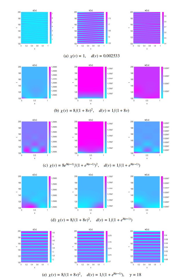
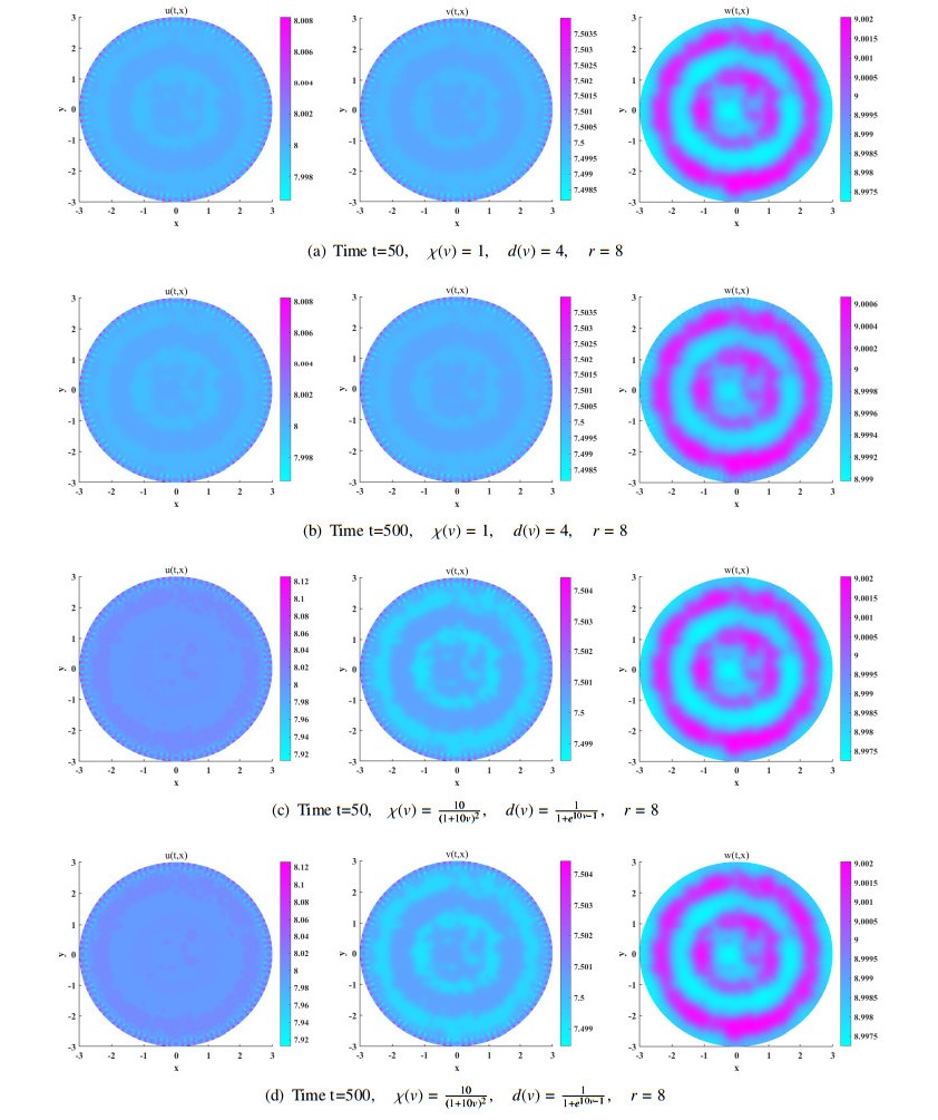
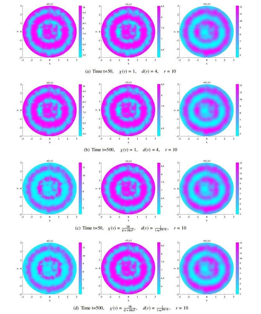
We study the existence of global unique classical solution to a density-dependent prey-predator population system with indirect prey-taxis effect. With two Lyapunov functions appropriately constructed, we then show that the solution can asymptotically approach prey-only state or coexistence state of the system under suitable conditions. Moreover, linearized analysis on the system at these two constant steady states shows their linear instability criterion. By numerical simulation we find that some density-dependent prey-taxis and predators' diffusion may either flatten the spatial one-dimensional patterns which exist in non-density-dependent case, or break the spatial two-dimensional distribution similarity which occurs in non-density-dependent case between predators and chemoattractants (released by prey).
Citation: Yong Luo. Global existence and stability of the classical solution to a density-dependent prey-predator model with indirect prey-taxis[J]. Mathematical Biosciences and Engineering, 2021, 18(5): 6672-6699. doi: 10.3934/mbe.2021331
We study the existence of global unique classical solution to a density-dependent prey-predator population system with indirect prey-taxis effect. With two Lyapunov functions appropriately constructed, we then show that the solution can asymptotically approach prey-only state or coexistence state of the system under suitable conditions. Moreover, linearized analysis on the system at these two constant steady states shows their linear instability criterion. By numerical simulation we find that some density-dependent prey-taxis and predators' diffusion may either flatten the spatial one-dimensional patterns which exist in non-density-dependent case, or break the spatial two-dimensional distribution similarity which occurs in non-density-dependent case between predators and chemoattractants (released by prey).

| [1] |
P. Kareiva, G. Odell, Swarms of predators exhibit "preytaxis" if individual predators use area-restricted search, Am. Naturalist, 130 (1987), 233–270. doi: 10.1086/284707

|
| [2] |
S. N. Wu, J. P. Shi, B. Y. Wu, Global existence of solutions and uniform persistence of a diffusive predator–prey model with prey-taxis, J. Differ. Equations, 260 (2016), 5847–5874. doi: 10.1016/j.jde.2015.12.024
|
| [3] | J. R. Beddington. Mutual interference between parasites or predators and its effect on searching efficiency, J. Anim. Ecol., 44 (1975), 331–340. |
| [4] |
D. L. DeAngelis, R. A. Goldstein, R. V. O'Neill, A model for tropic interaction, Ecology, 56 (1975), 881–892. doi: 10.2307/1936298
|
| [5] |
P. A. Abrams, L. R. Ginzburg, The nature of predation: prey dependent, ratio dependent or neither?, Trends Ecol. Evol., 15 (2000), 337–341. doi: 10.1016/S0169-5347(00)01908-X
|
| [6] |
H. Y. Jin, Z. A. Wang, Global stability of prey-taxis systems, J. Diffe. Equations, 262 (2017), 1257–1290. doi: 10.1016/j.jde.2016.10.010
|
| [7] | Y. L. Cai, Q. Cao, Z. A. Wang, Asymptotic dynamics and spatial patterns of a ratio-dependent predator–prey system with prey-taxis, Appl. Anal., (2020), 1–19. |
| [8] |
T. Hillen, K. Painter, Global existence for a parabolic chemotaxis model with prevention of overcrowding, Adv. Appl. Math., 26 (2001), 280–301. doi: 10.1006/aama.2001.0721
|
| [9] |
B. E. Ainseba, M. Bendahmane, A. Noussair, A reaction–diffusion system modeling predator–prey with prey-taxis, Nonlinear Anal. Real World Appl., 9 (2008), 2086–2105. doi: 10.1016/j.nonrwa.2007.06.017
|
| [10] |
Y. S. Tao, Global existence of classical solutions to a predator–prey model with nonlinear prey-taxis, Nonlinear Anal. Real World Appl., 11 (2010), 2056–2064. doi: 10.1016/j.nonrwa.2009.05.005
|
| [11] |
X. He, S. N. Zheng, Global boundedness of solutions in a reaction–diffusion system of predator–prey model with prey-taxis, Appl. Math. Lett., 49 (2015), 73–77. doi: 10.1016/j.aml.2015.04.017
|
| [12] |
C. L. Li, X. H. Wang, Y. F. Shao, Steady states of a predator–prey model with prey-taxis, Nonlinear Anal. Theory Meth. Appl., 97 (2014), 155–168. doi: 10.1016/j.na.2013.11.022
|
| [13] |
X. L. Wang, W. D. Wang, G. H. Zhang, Global bifurcation of solutions for a predator–prey model with prey-taxis, Math. Meth. Appl. Sci., 38 (2015), 431–443. doi: 10.1002/mma.3079
|
| [14] |
H. Y. Jin, Z. A. Wang, Global dynamics and spatio-temporal patterns of predator–prey systems with density-dependent motion, Eur. J. Appl. Math., 32 (2021), 652–682. doi: 10.1017/S0956792520000248
|
| [15] |
B. Roy, S. K. Roy, D. B. Gurung, Holling–Tanner model with Beddington–DeAngelis functional response and time delay introducing harvesting, Math. Comput. Simul., 142 (2017), 1–14. doi: 10.1016/j.matcom.2017.03.010
|
| [16] |
B. Roy, S. K. Roy, M. H. A. Biswas, Effects on prey–predator with different functional responses, Int. J. Biomath., 10 (2017), 1750113. doi: 10.1142/S1793524517501133
|
| [17] | A. Jana, S. K. Roy, Holling-Tanner prey-predator model with Beddington-DeAngelis functional response including delay, Int. J. Model. Simul., (2020), 1–15. |
| [18] |
S. K. Roy, B. Roy, Analysis of prey-predator three species fishery model with harvesting including prey refuge and migration, Int. J. Bifurcat. Chaos, 26 (2016), 1650022. doi: 10.1142/S021812741650022X
|
| [19] |
B. Roy, S. K. Roy, Analysis of prey-predator three species models with vertebral and invertebral predators, Int. J. Dyn. Control, 3 (2015), 306–312. doi: 10.1007/s40435-015-0153-6
|
| [20] |
J. I. Tello, D. Wrzosek, Predator–prey model with diffusion and indirect prey-taxis, Math. Models Methods Appl. Sci., 26 (2016), 2129–2162. doi: 10.1142/S0218202516400108
|
| [21] |
Y. V. Tyutyunov, L. I. Titova, I. N. Senina, Prey-taxis destabilizes homogeneous stationary state in spatial Gause– Kolmogorov-type model for predator–prey system, Ecol. Complex., 31 (2017), 170–180. doi: 10.1016/j.ecocom.2017.07.001
|
| [22] |
H. Y. Jin, S. J. Shi, Z. A. Wang, Boundedness and asymptotics of a reaction-diffusion system with density-dependent motility, J. Differ. Equations, 269 (2020), 6758–6793. doi: 10.1016/j.jde.2020.05.018
|
| [23] |
H. Y. Jin, Z. A. Wang, Critical mass on the Keller-Segel system with signal-dependent motility, P. Am. Math. Soc., 148 (2020), 4855–4873. doi: 10.1090/proc/15124
|
| [24] |
X. F. Fu, L. H. Tang, C. L. Liu, J. D. Huang, T. Hwa, P. Lenz, Stripe formation in bacterial systems with density-suppressed motility, Phys. Rev. Lett., 108 (2012), 198102. doi: 10.1103/PhysRevLett.108.198102
|
| [25] |
J. Smith-Roberge, D. Iron, T. Kolokolnikov, Pattern formation in bacterial colonies with density-dependent diffusion, Eur. J. Appl. Math., 30 (2019), 196–218. doi: 10.1017/S0956792518000013
|
| [26] |
H. Y. Jin, Y. J. Kim, Z. A. Wang, Boundedness, stabilization, and pattern formation driven by density-suppressed motility, SIAM J. Appl. Math., 78 (2018), 1632–1657. doi: 10.1137/17M1144647
|
| [27] |
S. L. Wang, J. F. Zhang, F. Xu, X. Y. Song, Dynamics of virus infection models with density-dependent diffusion, Comput. Math. Appl., 74 (2017), 2403–2422. doi: 10.1016/j.camwa.2017.07.019
|
| [28] | W. J. Zuo, Y. L. Song, Stability and double-Hopf bifurcations of a Gause-Kolmogorov-type predator–prey system with indirect prey-taxis, J. Dyn. Differ. Equations, (2020), 1–41. |
| [29] |
I. Ahn, C. Yoon, Global well-posedness and stability analysis of prey-predator model with indirect prey-taxis, J. Differ. Equations, 268 (2020), 4222–4255. doi: 10.1016/j.jde.2019.10.019
|
| [30] | J. P. Wang, M. X. Wang, The dynamics of a predator–prey model with diffusion and indirect prey-taxis, J. Dyn. Differ. Equations, 32 (2019), 1291–1310. |
| [31] | H. Amann, Dynamic theory of quasilinear parabolic equations. II. Reaction-diffusion systems, Differ. Integral Equations, 3 (1990), 13–75. |
| [32] |
H. Amann, Dynamic theory of quasilinear parabolic systems. III. Global existence, Math. Z., 202 (1989), 219–250. doi: 10.1007/BF01215256
|
| [33] | H. Amann, Linear and Quasilinear Parabolic Problems Volume I: Abstract Linear Theory, Monographs in Mathematics, Birkhäuser, Basel, 1995. |
| [34] |
R. Kowalczyk, Z. Szymańska, On the global existence of solutions to an aggregation model, J. Math. Anal. Appl., 343 (2008), 379–398. doi: 10.1016/j.jmaa.2008.01.005
|
| [35] | D. Henry, Geometric Theory of Semilinear Parabolic Equations, Lecture Notes in Mathematics, Springer-Verlag, Berlin Heidelberg, 1981. |
| [36] |
D. Horstmann, M. Winkler, Boundedness vs. blow-up in a chemotaxis system, J. Differ. Equations, 215 (2005), 52–107. doi: 10.1016/j.jde.2004.10.022
|
| [37] | O. A. Ladyzhenskaia, V. A. Solonnikov, N. N. Ural'tseva, Linear and Quasi-linear Equations of Parabolic Type, American Mathematical Society, 1968. |
| [38] |
J. R. Ellis, N. B. Petrovskaya, A computational study of density-dependent individual movement and the formation of population clusters in two-dimensional spatial domains, J. Theor. Biol., 505 (2020), 110421. doi: 10.1016/j.jtbi.2020.110421
|
Figures(3) / Tables(2)

Yong Luo. Global existence and stability of the classical solution to a density-dependent prey-predator model with indirect prey-taxis[J]. Mathematical Biosciences and Engineering, 2021, 18(5): 6672-6699. doi: 10.3934/mbe.2021331


 DownLoad: